---
title: Softmax
date: 2025-11-09T10:16:26Z
modified: 2026-06-29T06:52:26Z
permalink: "https://www.micheledpierri.com/2025/11/09/softmax-machine-learning/"
type: post
status: publish
excerpt: ""
wpid: 1044
categories:
  - Data Analysis
  - Machine Learning
  - Programming
tags:
  - Data Analysis
  - Machine Learning
  - Programming
  - Python
featured_image: "https://www.micheledpierri.com/wp-content/uploads/2025/11/softmax_.png"
featured_image_alt: Villagers and children in period clothing gaze upward as dozens of muted red, gold, blue, and cream balloons drift above a cobbled old European street in a warm, painterly historical scene.
timestamp: 2026-06-29T06:52:26Z
---

## Introduction

The softmax function is essential in mathematics and machine learning.

It transforms a vector of real numbers into a probability distribution.

Put simply, it converts a set of numbers into probabilities.

To understand how it works, let’s look at a list of risk values for some patients:


| Patients | Surgical Risk |
| --- | --- |
| Patient A | 2 |
| Patient B | 1 |
| Patient C |  |

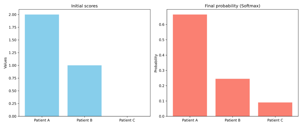
When we apply the softmax function to this series of numbers \[2,1,0\] we get:


| Patients | Surgical Risk |
| --- | --- |
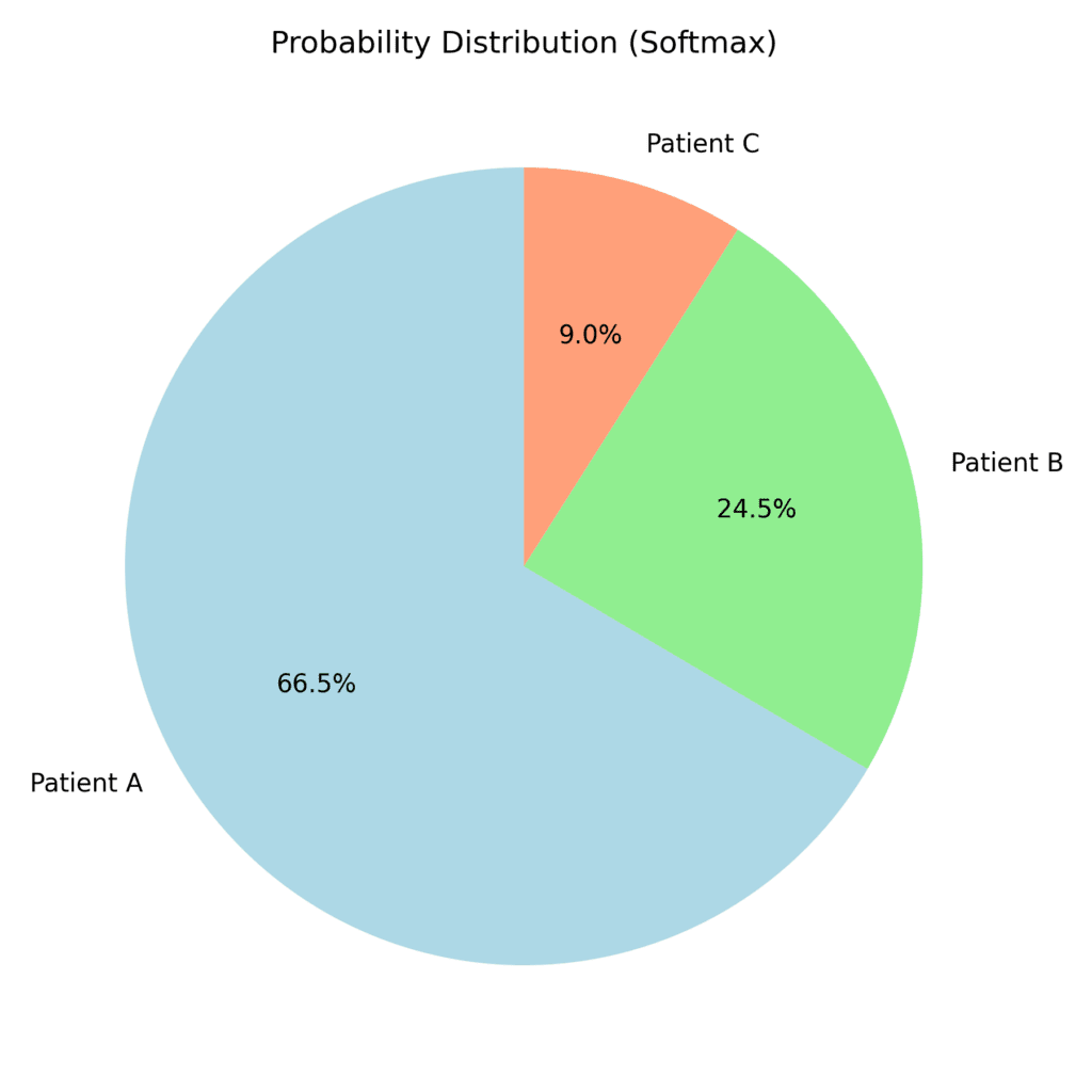
| Patient A | 66% (0.66) |
| Patient B | 24% (0.24) |
| Patient C | 9% (0.9) |

Note that the resulting probability values from the softmax function always sum to 1 (or 100%).

## How does it work?

The Softmax transformation consists of two key operations: exponentiation and normalization.

During exponentiation, we calculate e^x for each number. This amplifies larger numbers while reducing smaller ones in the series.

In the normalization step, we sum all the numbers and divide each by that total. This produces values between 0 and 1 that always sum to 1.

These two steps together create our final probability distribution.

The graphs illustrate how Softmax transforms numerical values into probabilities, with the resulting probabilities always summing to one.
![From initial scores to final probability bar graphs](https://www.micheledpierri.com/wp-content/uploads/2025/02/softmax_graphs_1-1024x427.png)

![Probability function with softmax](https://www.micheledpierri.com/wp-content/uploads/2025/02/softmax_graphs_2-1024x1024.png)

## Mathematical Formula for Softmax

For a vector z = \[z₁, z₂, z₃…zₙ\], the Softmax formula is:

![\text{softmax}(z_i) = \frac{e^{z_i}}{\sum_{j=1}^{n} e^{z_j}}](https://www.micheledpierri.com/wp-content/ql-cache/quicklatex.com-a213b1b7ba42644fa8a57eec33f62dc1_l3.svg "Rendered by QuickLaTeX.com")

Where: – ![z_i](https://www.micheledpierri.com/wp-content/ql-cache/quicklatex.com-035344d0858f49aa72f450dbd3704e4d_l3.svg "Rendered by QuickLaTeX.com") is the ![i](https://www.micheledpierri.com/wp-content/ql-cache/quicklatex.com-ca3f29ee5ba83c877b5b3cc14f47dbcb_l3.svg "Rendered by QuickLaTeX.com")

-th element of the input vector ![z](https://www.micheledpierri.com/wp-content/ql-cache/quicklatex.com-87a05c83ed14913d5d6c549466bac3de_l3.svg "Rendered by QuickLaTeX.com")

, – ![e^{z_i}](https://www.micheledpierri.com/wp-content/ql-cache/quicklatex.com-724c6ca78808b226386df7d66a0d5f3a_l3.svg "Rendered by QuickLaTeX.com") is the exponential of ![z_i](https://www.micheledpierri.com/wp-content/ql-cache/quicklatex.com-035344d0858f49aa72f450dbd3704e4d_l3.svg "Rendered by QuickLaTeX.com")

, – ![\sum_{j=1}^{n} e^{z_j}](https://www.micheledpierri.com/wp-content/ql-cache/quicklatex.com-c8484d95797b3910630ed6277fe1e6d5_l3.svg "Rendered by QuickLaTeX.com") is the sum of the exponentials of all elements in the vector ![z](https://www.micheledpierri.com/wp-content/ql-cache/quicklatex.com-87a05c83ed14913d5d6c549466bac3de_l3.svg "Rendered by QuickLaTeX.com")

, – ![n](https://www.micheledpierri.com/wp-content/ql-cache/quicklatex.com-aee4c0f630649ac4f2d99ff70c000710_l3.svg "Rendered by QuickLaTeX.com") is the total number of elements in the vector ![z](https://www.micheledpierri.com/wp-content/ql-cache/quicklatex.com-87a05c83ed14913d5d6c549466bac3de_l3.svg "Rendered by QuickLaTeX.com")

. This formula ensures that each output value lies between 0 and 1, and the sum of all outputs equals 1.

​

## Graphical Examples of Softmax

For two classes, the Softmax function simplifies to a sigmoid function, where the first class has probability p1 and the second class has probability 1-p1 (since probabilities must sum to 1). As one class’s probability increases, the other’s must decrease proportionally.

![Softmax function for two classes](https://www.micheledpierri.com/wp-content/uploads/2025/02/softmax_2_classi-1024x768.png)

For three classes, we can visualize the function using a three-dimensional graph. When we treat the first two classes as variables and fix the third as a constant, the graph displays the probabilities of the first two classes. The third class’s probability is then calculated as 1 minus the sum of the first two class probabilities.

![Softmax function for three classes](https://www.micheledpierri.com/wp-content/uploads/2025/02/softmax_3_classi-1024x683.png)

### Numerical Saturation and Normalization by Maximum

A key challenge when applying the Softmax function occurs with extremely large or small z values.

These extreme values can cause overflow or underflow—situations where numbers become too large or too small for a computer to represent accurately.

Consider a vector z with large numbers:

z=\[1000, 1001, 1002\]

​Calculating ![e^{1000}](https://www.micheledpierri.com/wp-content/ql-cache/quicklatex.com-20277a9b17c568a97f75868531ff3f76_l3.svg "Rendered by QuickLaTeX.com")

, ![e^{1001}](https://www.micheledpierri.com/wp-content/ql-cache/quicklatex.com-3a52b7bd1abf41b7a85023ca02222ddc_l3.svg "Rendered by QuickLaTeX.com")

, and ![e^{1002}](https://www.micheledpierri.com/wp-content/ql-cache/quicklatex.com-6646eeaaa753322605cae6bdbbdf263b_l3.svg "Rendered by QuickLaTeX.com") for Softmax would produce enormous numbers that cause overflow.

To solve this, we can normalize the vector. The new vector z’ then has much smaller values:

z’ = \[1000 – 1002, 1001 – 1002, 1002 – 1002\] = \[-2, -1, 0\]

​This normalization gives us manageable exponential values:

![e^{-2} \approx 0.135, \quad e^{-1} \approx 0.368, \quad e^{0} = 1](https://www.micheledpierri.com/wp-content/ql-cache/quicklatex.com-ec570c3225ca720a1bc36ba8280e91d0_l3.svg "Rendered by QuickLaTeX.com")

​Finally, we calculate the sum of exponentials and apply the softmax function:

![\text{Sum} = 0.135 + 0.368 + 1 = 1.503](https://www.micheledpierri.com/wp-content/ql-cache/quicklatex.com-c6c5923db4cdc44a56682976b52d468a_l3.svg "Rendered by QuickLaTeX.com")


![\text{Softmax} = \left[\frac{0.135}{1.503}, \frac{0.368}{1.503}, \frac{1}{1.503}\right] \approx [0.09, 0.24, 0.67]](https://www.micheledpierri.com/wp-content/ql-cache/quicklatex.com-94c1754c5750e6a6cd4727722d1861a9_l3.svg "Rendered by QuickLaTeX.com")

​

This same approach works for very small z values.

For both extremely large and small values, we can use a modified formula:

![\text{softmax}(z_i) = \frac{e^{z_i - \max(z)}}{\sum_{j=1}^{n} e^{z_j - \max(z)}}](https://www.micheledpierri.com/wp-content/ql-cache/quicklatex.com-5f84b7757d21f5b06264a2fff0e5e96e_l3.svg "Rendered by QuickLaTeX.com")

​

## Softmax with Python

Let’s explore how to implement the Softmax function in Python, covering both single vector applications and matrix operations.

# Example of applying softmax to a NumPy array

import numpy as np

def softmax(z):
    # Subtract maximum value to prevent numerical overflow
    z = z - np.max(z)
    exp_z = np.exp(z)
    return exp_z / np.sum(exp_z)

# Example usage
z = np.array([2.0, 1.0, 0.1])
print("Input:", z)
print("Softmax Output:", softmax(z))```
<span class="line"><span style="color: #6272A4"># Example of applying softmax to a NumPy array</span></span>
<span class="line"></span>
<span class="line"><span style="color: #FF79C6">import</span><span style="color: #F8F8F2"> numpy </span><span style="color: #FF79C6">as</span><span style="color: #F8F8F2"> np</span></span>
<span class="line"></span>
<span class="line"><span style="color: #FF79C6">def</span><span style="color: #F8F8F2"> </span><span style="color: #50FA7B">softmax</span><span style="color: #F8F8F2">(</span><span style="color: #FFB86C; font-style: italic">z</span><span style="color: #F8F8F2">):</span></span>
<span class="line"><span style="color: #F8F8F2">    </span><span style="color: #6272A4"># Subtract maximum value to prevent numerical overflow</span></span>
<span class="line"><span style="color: #F8F8F2">    z </span><span style="color: #FF79C6">=</span><span style="color: #F8F8F2"> z </span><span style="color: #FF79C6">-</span><span style="color: #F8F8F2"> np.max(z)</span></span>
<span class="line"><span style="color: #F8F8F2">    exp_z </span><span style="color: #FF79C6">=</span><span style="color: #F8F8F2"> np.exp(z)</span></span>
<span class="line"><span style="color: #F8F8F2">    </span><span style="color: #FF79C6">return</span><span style="color: #F8F8F2"> exp_z </span><span style="color: #FF79C6">/</span><span style="color: #F8F8F2"> np.sum(exp_z)</span></span>
<span class="line"></span>
<span class="line"><span style="color: #6272A4"># Example usage</span></span>
<span class="line"><span style="color: #F8F8F2">z </span><span style="color: #FF79C6">=</span><span style="color: #F8F8F2"> np.array([</span><span style="color: #BD93F9">2.0</span><span style="color: #F8F8F2">, </span><span style="color: #BD93F9">1.0</span><span style="color: #F8F8F2">, </span><span style="color: #BD93F9">0.1</span><span style="color: #F8F8F2">])</span></span>
<span class="line"><span style="color: #8BE9FD">print</span><span style="color: #F8F8F2">(</span><span style="color: #E9F284">"</span><span style="color: #F1FA8C">Input:</span><span style="color: #E9F284">"</span><span style="color: #F8F8F2">, z)</span></span>
<span class="line"><span style="color: #8BE9FD">print</span><span style="color: #F8F8F2">(</span><span style="color: #E9F284">"</span><span style="color: #F1FA8C">Softmax Output:</span><span style="color: #E9F284">"</span><span style="color: #F8F8F2">, softmax(z))</span></span>
```

# Matrix application example

def softmax_batch(z):
    # Subtract the maximum along axis 1 (per row)
    z = z - np.max(z, axis=1, keepdims=True)
    exp_z = np.exp(z)
    return exp_z / np.sum(exp_z, axis=1, keepdims=True)

# Usage example
z_batch = np.array([[2.0, 1.0, 0.1], [1.0, 2.0, 3.0]])
print("Input Batch:\n", z_batch)
print("Softmax Output Batch:\n", softmax_batch(z_batch))```
<span class="line"><span style="color: #6272A4"># Matrix application example</span></span>
<span class="line"></span>
<span class="line"><span style="color: #FF79C6">def</span><span style="color: #F8F8F2"> </span><span style="color: #50FA7B">softmax_batch</span><span style="color: #F8F8F2">(</span><span style="color: #FFB86C; font-style: italic">z</span><span style="color: #F8F8F2">):</span></span>
<span class="line"><span style="color: #F8F8F2">    </span><span style="color: #6272A4"># Subtract the maximum along axis 1 (per row)</span></span>
<span class="line"><span style="color: #F8F8F2">    z </span><span style="color: #FF79C6">=</span><span style="color: #F8F8F2"> z </span><span style="color: #FF79C6">-</span><span style="color: #F8F8F2"> np.max(z, </span><span style="color: #FFB86C; font-style: italic">axis</span><span style="color: #FF79C6">=</span><span style="color: #BD93F9">1</span><span style="color: #F8F8F2">, </span><span style="color: #FFB86C; font-style: italic">keepdims</span><span style="color: #FF79C6">=</span><span style="color: #BD93F9">True</span><span style="color: #F8F8F2">)</span></span>
<span class="line"><span style="color: #F8F8F2">    exp_z </span><span style="color: #FF79C6">=</span><span style="color: #F8F8F2"> np.exp(z)</span></span>
<span class="line"><span style="color: #F8F8F2">    </span><span style="color: #FF79C6">return</span><span style="color: #F8F8F2"> exp_z </span><span style="color: #FF79C6">/</span><span style="color: #F8F8F2"> np.sum(exp_z, </span><span style="color: #FFB86C; font-style: italic">axis</span><span style="color: #FF79C6">=</span><span style="color: #BD93F9">1</span><span style="color: #F8F8F2">, </span><span style="color: #FFB86C; font-style: italic">keepdims</span><span style="color: #FF79C6">=</span><span style="color: #BD93F9">True</span><span style="color: #F8F8F2">)</span></span>
<span class="line"></span>
<span class="line"><span style="color: #6272A4"># Usage example</span></span>
<span class="line"><span style="color: #F8F8F2">z_batch </span><span style="color: #FF79C6">=</span><span style="color: #F8F8F2"> np.array([[</span><span style="color: #BD93F9">2.0</span><span style="color: #F8F8F2">, </span><span style="color: #BD93F9">1.0</span><span style="color: #F8F8F2">, </span><span style="color: #BD93F9">0.1</span><span style="color: #F8F8F2">], [</span><span style="color: #BD93F9">1.0</span><span style="color: #F8F8F2">, </span><span style="color: #BD93F9">2.0</span><span style="color: #F8F8F2">, </span><span style="color: #BD93F9">3.0</span><span style="color: #F8F8F2">]])</span></span>
<span class="line"><span style="color: #8BE9FD">print</span><span style="color: #F8F8F2">(</span><span style="color: #E9F284">"</span><span style="color: #F1FA8C">Input Batch:</span><span style="color: #FF79C6">\n</span><span style="color: #E9F284">"</span><span style="color: #F8F8F2">, z_batch)</span></span>
<span class="line"><span style="color: #8BE9FD">print</span><span style="color: #F8F8F2">(</span><span style="color: #E9F284">"</span><span style="color: #F1FA8C">Softmax Output Batch:</span><span style="color: #FF79C6">\n</span><span style="color: #E9F284">"</span><span style="color: #F8F8F2">, softmax_batch(z_batch))</span></span>
```

​

## Applications

The Softmax function has three main applications:

In Multiclass Classification (Machine Learning): It converts raw scores into a probability distribution across possible classes

In Neural Networks: It serves as the activation function in the output layer

In Reinforcement Learning: It transforms action scores into selection probabilities

## Conclusion

The Softmax function plays a vital role in machine learning, especially for multiclass classification tasks. Its mathematical properties and computational efficiency have made it indispensable in neural networks and predictive models. Proper implementation and careful handling of numerical challenges are key to achieving optimal results.