---
title: Non-Parametric Statistics in Medicine
date: 2026-05-19T11:30:34Z
modified: 2026-05-19T11:30:39Z
permalink: "https://www.micheledpierri.com/2026/05/19/non-parametric-statistics-in-medicine/"
type: post
status: publish
excerpt: ""
wpid: 2745
categories:
  - Data Analysis
  - Statistics
tags:
  - Data Analysis
  - Statistics
  - Data Science
  - Python
featured_image: "https://www.micheledpierri.com/wp-content/uploads/2026/05/nonparametric.png"
featured_image_alt: People climb a staircase with uneven steps
timestamp: 2026-05-19T11:30:39Z
---

## **Non-Parametric Statistics in Medicine:** 

_**A Practical Guide for Skewed, Ordinal, and Small Clinical Datasets**_

Last updated: May 2026

Author: Michele D. Pierri

Reading time: 15–20 minutes

---

## Introduction

Clinical data rarely behave like the textbook examples we encounter in introductory statistics courses. Length of stay tends to be right-skewed. Biomarkers such as C-reactive protein, ferritin, D-dimer, troponin, or NT-proBNP frequently show extreme values, sometimes by an order of magnitude. Pain scores and functional classes are bounded, discrete, partly ordinal. And pilot studies, which most of us run at some point in our careers, often involve small samples where a single outlier can drag the mean in a misleading direction.

For these reasons, non-parametric statistics should not be viewed as a secondary or somehow inferior form of analysis. In many clinical scenarios, they are simply the most coherent statistical choice available.

The key idea is straightforward:

> Non-parametric tests are useful when the clinical variable is ordinal, markedly skewed, affected by outliers, or when the assumptions required by classical parametric tests are not clinically or statistically convincing.

That said, non-parametric statistics should not be reduced to the simplistic rule:

> “If the Shapiro-Wilk test is significant, use a non-parametric test.”

This rule is incomplete and, in our clinical experience, sometimes misleading. The real question is not only whether the data are normally distributed. The real question is whether the statistical method matches the clinical structure of the data, the study design, and the interpretation we want to make.

In this article we will walk through four simulated clinical scenarios:

1. Pain before and after treatment: **Wilcoxon signed-rank test**
2. Length of stay in two independent groups: **Mann-Whitney U test**
3. Biomarker levels across three clinical groups: **Kruskal-Wallis test**
4. Repeated ordinal clinical scores over time: **Friedman test**

The examples are intentionally simple. Their purpose is not to replace a full statistical analysis plan but to show how non-parametric thinking works in realistic medical situations.

> ## Quick cheat sheet (clinical workflow)
> 
> - **Summarize** skewed continuous variables as median (IQR); ordinal variables as median (IQR) or category counts when appropriate.
> - **Match design to test**: paired → Wilcoxon; 2 independent groups → Mann-Whitney; >2 independent groups → Kruskal-Wallis; repeated measures (ordinal/ranked) → Friedman.
> - **Report beyond p-values**: an effect size with confidence interval (or at least an effect size), and a clinically interpretable difference (e.g., median change).
> - **Plan post-hoc**: if Kruskal-Wallis or Friedman is significant, use corrected pairwise comparisons (e.g., Holm or Benjamini-Hochberg).

---

## 1. What Does “Non-Parametric” Mean?

Parametric tests, such as the t-test or ANOVA, usually rely on assumptions about the distribution of the data or the distribution of model residuals. They typically focus on means and standard deviations.

Non-parametric tests, by contrast, require fewer distributional assumptions. Many of them work by replacing raw values with their **ranks**.

Consider, instead of comparing the exact length of stay values:

5, 6, 7, 8, 35
```
<span class="line"><span style="color: #50FA7B">5,</span><span style="color: #F8F8F2"> </span><span style="color: #BD93F9">6</span><span style="color: #F1FA8C">,</span><span style="color: #F8F8F2"> </span><span style="color: #BD93F9">7</span><span style="color: #F1FA8C">,</span><span style="color: #F8F8F2"> </span><span style="color: #BD93F9">8</span><span style="color: #F1FA8C">,</span><span style="color: #F8F8F2"> </span><span style="color: #BD93F9">35</span></span>
<span class="line"></span>
```

A rank-based method asks where each patient stands relative to the others. This simple reframing makes the method far less sensitive to extreme values.

It does not mean, however, that non-parametric tests have no assumptions at all. They still require appropriate study design, independent observations when required, and correct pairing when the data are paired. They also answer specific statistical questions that are not always identical to their parametric counterparts.

One particularly important point deserves emphasis:

> The Mann-Whitney U test is often described as a test comparing medians, but this is strictly valid only under specific distributional conditions. More generally, it tests whether values from one group tend to be larger or smaller than values from another group.

This distinction matters a great deal in clinical writing, even if it is routinely glossed over.

---

## Scenario 1: Pain Before and After Treatment

## Clinical question

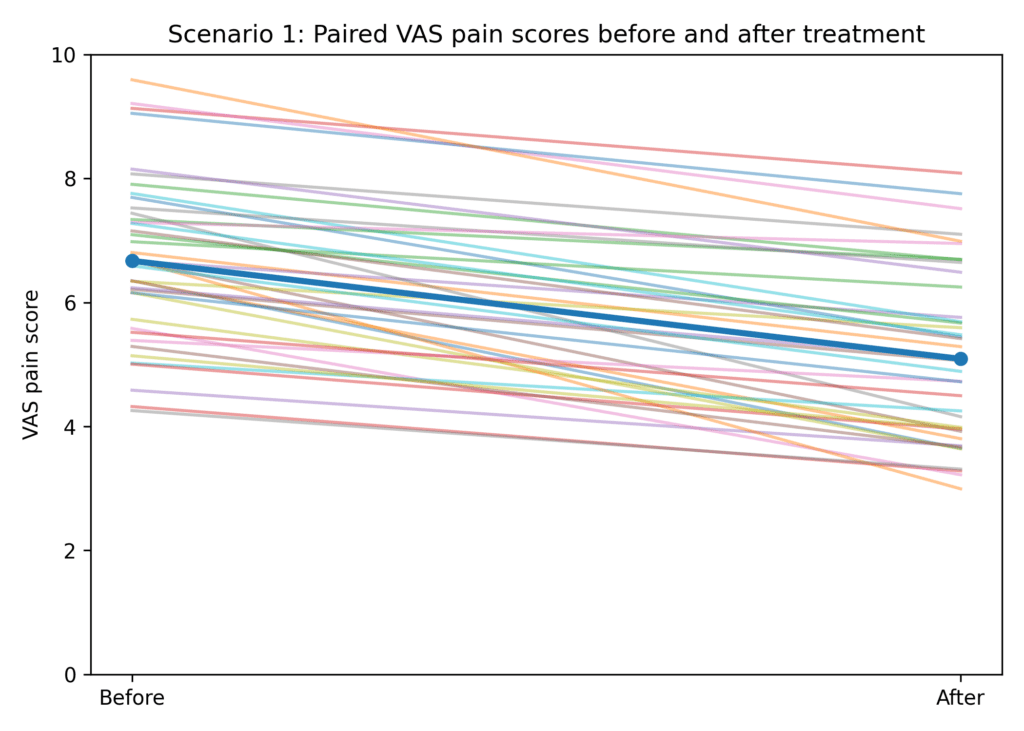
A group of patients with chronic low back pain receives a new analgesic treatment. Pain is measured using a Visual Analogue Scale (VAS) from 0 to 10, both before and after treatment.

The question is:

> Did pain decrease after treatment?

## Why a non-parametric test may be appropriate

VAS scores are bounded between 0 and 10. They are frequently not normally distributed. Anyone who has collected VAS data in clinic knows the typical clustering at specific values (0, 5, 8, or 10). The data are also paired: each patient has a before-treatment and after-treatment value.

The appropriate non-parametric test is the **Wilcoxon signed-rank test**.

It is the non-parametric analogue of the paired t-test, although the interpretation is not exactly the same. It evaluates whether paired differences are symmetrically distributed around zero.

**Practical assumptions to check**

- Correct pairing (each “before” matches the same patient “after”).
- Differences are roughly symmetric around a central value (often 0). If differences are extremely skewed, consider alternative approaches such as the sign test or a model-based strategy.

## Basic Python example

import numpy as np
import pandas as pd
from scipy.stats import wilcoxon

np.random.seed(42)

n = 40

pain_before = np.clip(np.random.normal(loc=7.0, scale=1.4, size=n), 0, 10)
improvement = np.random.gamma(shape=2.0, scale=0.8, size=n)
pain_after = np.clip(pain_before - improvement, 0, 10)

data_pain = pd.DataFrame({
    "patient_id": range(1, n + 1),
    "pain_before": pain_before,
    "pain_after": pain_after
})

stat, p_value = wilcoxon(data_pain["pain_before"], data_pain["pain_after"])

print(data_pain.head())
print(f"Wilcoxon statistic:{stat:.3f}")
print(f"p-value:{p_value:.4f}")
```
<span class="line"><span style="color: #FF79C6">import</span><span style="color: #F8F8F2"> numpy </span><span style="color: #FF79C6">as</span><span style="color: #F8F8F2"> np</span></span>
<span class="line"><span style="color: #FF79C6">import</span><span style="color: #F8F8F2"> pandas </span><span style="color: #FF79C6">as</span><span style="color: #F8F8F2"> pd</span></span>
<span class="line"><span style="color: #FF79C6">from</span><span style="color: #F8F8F2"> scipy.stats </span><span style="color: #FF79C6">import</span><span style="color: #F8F8F2"> wilcoxon</span></span>
<span class="line"></span>
<span class="line"><span style="color: #F8F8F2">np.random.seed(</span><span style="color: #BD93F9">42</span><span style="color: #F8F8F2">)</span></span>
<span class="line"></span>
<span class="line"><span style="color: #F8F8F2">n </span><span style="color: #FF79C6">=</span><span style="color: #F8F8F2"> </span><span style="color: #BD93F9">40</span></span>
<span class="line"></span>
<span class="line"><span style="color: #F8F8F2">pain_before </span><span style="color: #FF79C6">=</span><span style="color: #F8F8F2"> np.clip(np.random.normal(</span><span style="color: #FFB86C; font-style: italic">loc</span><span style="color: #FF79C6">=</span><span style="color: #BD93F9">7.0</span><span style="color: #F8F8F2">, </span><span style="color: #FFB86C; font-style: italic">scale</span><span style="color: #FF79C6">=</span><span style="color: #BD93F9">1.4</span><span style="color: #F8F8F2">, </span><span style="color: #FFB86C; font-style: italic">size</span><span style="color: #FF79C6">=</span><span style="color: #F8F8F2">n), </span><span style="color: #BD93F9">0</span><span style="color: #F8F8F2">, </span><span style="color: #BD93F9">10</span><span style="color: #F8F8F2">)</span></span>
<span class="line"><span style="color: #F8F8F2">improvement </span><span style="color: #FF79C6">=</span><span style="color: #F8F8F2"> np.random.gamma(</span><span style="color: #FFB86C; font-style: italic">shape</span><span style="color: #FF79C6">=</span><span style="color: #BD93F9">2.0</span><span style="color: #F8F8F2">, </span><span style="color: #FFB86C; font-style: italic">scale</span><span style="color: #FF79C6">=</span><span style="color: #BD93F9">0.8</span><span style="color: #F8F8F2">, </span><span style="color: #FFB86C; font-style: italic">size</span><span style="color: #FF79C6">=</span><span style="color: #F8F8F2">n)</span></span>
<span class="line"><span style="color: #F8F8F2">pain_after </span><span style="color: #FF79C6">=</span><span style="color: #F8F8F2"> np.clip(pain_before </span><span style="color: #FF79C6">-</span><span style="color: #F8F8F2"> improvement, </span><span style="color: #BD93F9">0</span><span style="color: #F8F8F2">, </span><span style="color: #BD93F9">10</span><span style="color: #F8F8F2">)</span></span>
<span class="line"></span>
<span class="line"><span style="color: #F8F8F2">data_pain </span><span style="color: #FF79C6">=</span><span style="color: #F8F8F2"> pd.DataFrame({</span></span>
<span class="line"><span style="color: #F8F8F2">    </span><span style="color: #E9F284">"</span><span style="color: #F1FA8C">patient_id</span><span style="color: #E9F284">"</span><span style="color: #F8F8F2">: </span><span style="color: #8BE9FD">range</span><span style="color: #F8F8F2">(</span><span style="color: #BD93F9">1</span><span style="color: #F8F8F2">, n </span><span style="color: #FF79C6">+</span><span style="color: #F8F8F2"> </span><span style="color: #BD93F9">1</span><span style="color: #F8F8F2">),</span></span>
<span class="line"><span style="color: #F8F8F2">    </span><span style="color: #E9F284">"</span><span style="color: #F1FA8C">pain_before</span><span style="color: #E9F284">"</span><span style="color: #F8F8F2">: pain_before,</span></span>
<span class="line"><span style="color: #F8F8F2">    </span><span style="color: #E9F284">"</span><span style="color: #F1FA8C">pain_after</span><span style="color: #E9F284">"</span><span style="color: #F8F8F2">: pain_after</span></span>
<span class="line"><span style="color: #F8F8F2">})</span></span>
<span class="line"></span>
<span class="line"><span style="color: #F8F8F2">stat, p_value </span><span style="color: #FF79C6">=</span><span style="color: #F8F8F2"> wilcoxon(data_pain[</span><span style="color: #E9F284">"</span><span style="color: #F1FA8C">pain_before</span><span style="color: #E9F284">"</span><span style="color: #F8F8F2">], data_pain[</span><span style="color: #E9F284">"</span><span style="color: #F1FA8C">pain_after</span><span style="color: #E9F284">"</span><span style="color: #F8F8F2">])</span></span>
<span class="line"></span>
<span class="line"><span style="color: #8BE9FD">print</span><span style="color: #F8F8F2">(data_pain.head())</span></span>
<span class="line"><span style="color: #8BE9FD">print</span><span style="color: #F8F8F2">(</span><span style="color: #FF79C6">f</span><span style="color: #F1FA8C">"Wilcoxon statistic:</span><span style="color: #BD93F9">{</span><span style="color: #F8F8F2">stat</span><span style="color: #FF79C6">:.3f</span><span style="color: #BD93F9">}</span><span style="color: #F1FA8C">"</span><span style="color: #F8F8F2">)</span></span>
<span class="line"><span style="color: #8BE9FD">print</span><span style="color: #F8F8F2">(</span><span style="color: #FF79C6">f</span><span style="color: #F1FA8C">"p-value:</span><span style="color: #BD93F9">{</span><span style="color: #F8F8F2">p_value</span><span style="color: #FF79C6">:.4f</span><span style="color: #BD93F9">}</span><span style="color: #F1FA8C">"</span><span style="color: #F8F8F2">)</span></span>
<span class="line"></span>
```

![Graph showing paired VAS pain scores before and after treatment](https://www.micheledpierri.com/wp-content/uploads/2026/05/scenario_1_pain_before_after-1024x731.png)

## Interpretation

If the p-value falls below the chosen significance threshold, we conclude that the post-treatment pain scores differ from the pre-treatment scores in a statistically meaningful way.

Statistical significance, however, is not enough. A reduction of 0.3 points on a VAS scale may be statistically significant in a large sample yet clinically trivial. For this reason the analysis should always report the median change together with its interquartile range.

A reasonable reporting sentence might read:

> Pain decreased after treatment, with median VAS changing from 7.1 before treatment to 5.3 after treatment. The reduction was statistically significant according to the Wilcoxon signed-rank test.

---

## Scenario 2: Length of Stay in Two Independent Groups

## Clinical question

A cardiac surgery team wants to compare postoperative length of stay between patients with preoperative anemia and patients without preoperative anemia.

The question is:

> Is postoperative length of stay different between the two groups?

## Why a non-parametric test may be appropriate

Length of stay is rarely normally distributed. Most patients are discharged after a relatively short period. A handful of patients, however, remain hospitalized for considerably longer, often because of complications, frailty, infections, or prolonged rehabilitation needs.

The net result is a right-skewed distribution, sometimes severely so.

In this scenario the two groups are independent. The appropriate non-parametric test is the **Mann-Whitney U test**.

**Practical assumptions to check**

- Independence between groups (no repeated measurements of the same patient across groups).
- The variable is at least ordinal or continuous, and comparable across groups.

## Basic Python example

import numpy as np
import pandas as pd
from scipy.stats import mannwhitneyu

np.random.seed(42)

n_non_anemic = 55
n_anemic = 50

los_non_anemic = np.random.lognormal(mean=1.8, sigma=0.35, size=n_non_anemic)
los_anemic = np.random.lognormal(mean=2.05, sigma=0.45, size=n_anemic)

data_los = pd.DataFrame({
    "group": ["Non-anemic"] * n_non_anemic + ["Anemic"] * n_anemic,
    "length_of_stay": np.concatenate([los_non_anemic, los_anemic])
})

stat, p_value = mannwhitneyu(
    data_los.loc[data_los["group"] == "Non-anemic", "length_of_stay"],
    data_los.loc[data_los["group"] == "Anemic", "length_of_stay"],
    alternative="two-sided"
)

print(data_los.groupby("group")["length_of_stay"].median())
print(f"Mann-Whitney U statistic:{stat:.3f}")
print(f"p-value:{p_value:.4f}")
```
<span class="line"><span style="color: #FF79C6">import</span><span style="color: #F8F8F2"> numpy </span><span style="color: #FF79C6">as</span><span style="color: #F8F8F2"> np</span></span>
<span class="line"><span style="color: #FF79C6">import</span><span style="color: #F8F8F2"> pandas </span><span style="color: #FF79C6">as</span><span style="color: #F8F8F2"> pd</span></span>
<span class="line"><span style="color: #FF79C6">from</span><span style="color: #F8F8F2"> scipy.stats </span><span style="color: #FF79C6">import</span><span style="color: #F8F8F2"> mannwhitneyu</span></span>
<span class="line"></span>
<span class="line"><span style="color: #F8F8F2">np.random.seed(</span><span style="color: #BD93F9">42</span><span style="color: #F8F8F2">)</span></span>
<span class="line"></span>
<span class="line"><span style="color: #F8F8F2">n_non_anemic </span><span style="color: #FF79C6">=</span><span style="color: #F8F8F2"> </span><span style="color: #BD93F9">55</span></span>
<span class="line"><span style="color: #F8F8F2">n_anemic </span><span style="color: #FF79C6">=</span><span style="color: #F8F8F2"> </span><span style="color: #BD93F9">50</span></span>
<span class="line"></span>
<span class="line"><span style="color: #F8F8F2">los_non_anemic </span><span style="color: #FF79C6">=</span><span style="color: #F8F8F2"> np.random.lognormal(</span><span style="color: #FFB86C; font-style: italic">mean</span><span style="color: #FF79C6">=</span><span style="color: #BD93F9">1.8</span><span style="color: #F8F8F2">, </span><span style="color: #FFB86C; font-style: italic">sigma</span><span style="color: #FF79C6">=</span><span style="color: #BD93F9">0.35</span><span style="color: #F8F8F2">, </span><span style="color: #FFB86C; font-style: italic">size</span><span style="color: #FF79C6">=</span><span style="color: #F8F8F2">n_non_anemic)</span></span>
<span class="line"><span style="color: #F8F8F2">los_anemic </span><span style="color: #FF79C6">=</span><span style="color: #F8F8F2"> np.random.lognormal(</span><span style="color: #FFB86C; font-style: italic">mean</span><span style="color: #FF79C6">=</span><span style="color: #BD93F9">2.05</span><span style="color: #F8F8F2">, </span><span style="color: #FFB86C; font-style: italic">sigma</span><span style="color: #FF79C6">=</span><span style="color: #BD93F9">0.45</span><span style="color: #F8F8F2">, </span><span style="color: #FFB86C; font-style: italic">size</span><span style="color: #FF79C6">=</span><span style="color: #F8F8F2">n_anemic)</span></span>
<span class="line"></span>
<span class="line"><span style="color: #F8F8F2">data_los </span><span style="color: #FF79C6">=</span><span style="color: #F8F8F2"> pd.DataFrame({</span></span>
<span class="line"><span style="color: #F8F8F2">    </span><span style="color: #E9F284">"</span><span style="color: #F1FA8C">group</span><span style="color: #E9F284">"</span><span style="color: #F8F8F2">: [</span><span style="color: #E9F284">"</span><span style="color: #F1FA8C">Non-anemic</span><span style="color: #E9F284">"</span><span style="color: #F8F8F2">] </span><span style="color: #FF79C6">*</span><span style="color: #F8F8F2"> n_non_anemic </span><span style="color: #FF79C6">+</span><span style="color: #F8F8F2"> [</span><span style="color: #E9F284">"</span><span style="color: #F1FA8C">Anemic</span><span style="color: #E9F284">"</span><span style="color: #F8F8F2">] </span><span style="color: #FF79C6">*</span><span style="color: #F8F8F2"> n_anemic,</span></span>
<span class="line"><span style="color: #F8F8F2">    </span><span style="color: #E9F284">"</span><span style="color: #F1FA8C">length_of_stay</span><span style="color: #E9F284">"</span><span style="color: #F8F8F2">: np.concatenate([los_non_anemic, los_anemic])</span></span>
<span class="line"><span style="color: #F8F8F2">})</span></span>
<span class="line"></span>
<span class="line"><span style="color: #F8F8F2">stat, p_value </span><span style="color: #FF79C6">=</span><span style="color: #F8F8F2"> mannwhitneyu(</span></span>
<span class="line"><span style="color: #F8F8F2">    data_los.loc[data_los[</span><span style="color: #E9F284">"</span><span style="color: #F1FA8C">group</span><span style="color: #E9F284">"</span><span style="color: #F8F8F2">] </span><span style="color: #FF79C6">==</span><span style="color: #F8F8F2"> </span><span style="color: #E9F284">"</span><span style="color: #F1FA8C">Non-anemic</span><span style="color: #E9F284">"</span><span style="color: #F8F8F2">, </span><span style="color: #E9F284">"</span><span style="color: #F1FA8C">length_of_stay</span><span style="color: #E9F284">"</span><span style="color: #F8F8F2">],</span></span>
<span class="line"><span style="color: #F8F8F2">    data_los.loc[data_los[</span><span style="color: #E9F284">"</span><span style="color: #F1FA8C">group</span><span style="color: #E9F284">"</span><span style="color: #F8F8F2">] </span><span style="color: #FF79C6">==</span><span style="color: #F8F8F2"> </span><span style="color: #E9F284">"</span><span style="color: #F1FA8C">Anemic</span><span style="color: #E9F284">"</span><span style="color: #F8F8F2">, </span><span style="color: #E9F284">"</span><span style="color: #F1FA8C">length_of_stay</span><span style="color: #E9F284">"</span><span style="color: #F8F8F2">],</span></span>
<span class="line"><span style="color: #F8F8F2">    </span><span style="color: #FFB86C; font-style: italic">alternative</span><span style="color: #FF79C6">=</span><span style="color: #E9F284">"</span><span style="color: #F1FA8C">two-sided</span><span style="color: #E9F284">"</span></span>
<span class="line"><span style="color: #F8F8F2">)</span></span>
<span class="line"></span>
<span class="line"><span style="color: #8BE9FD">print</span><span style="color: #F8F8F2">(data_los.groupby(</span><span style="color: #E9F284">"</span><span style="color: #F1FA8C">group</span><span style="color: #E9F284">"</span><span style="color: #F8F8F2">)[</span><span style="color: #E9F284">"</span><span style="color: #F1FA8C">length_of_stay</span><span style="color: #E9F284">"</span><span style="color: #F8F8F2">].median())</span></span>
<span class="line"><span style="color: #8BE9FD">print</span><span style="color: #F8F8F2">(</span><span style="color: #FF79C6">f</span><span style="color: #F1FA8C">"Mann-Whitney U statistic:</span><span style="color: #BD93F9">{</span><span style="color: #F8F8F2">stat</span><span style="color: #FF79C6">:.3f</span><span style="color: #BD93F9">}</span><span style="color: #F1FA8C">"</span><span style="color: #F8F8F2">)</span></span>
<span class="line"><span style="color: #8BE9FD">print</span><span style="color: #F8F8F2">(</span><span style="color: #FF79C6">f</span><span style="color: #F1FA8C">"p-value:</span><span style="color: #BD93F9">{</span><span style="color: #F8F8F2">p_value</span><span style="color: #FF79C6">:.4f</span><span style="color: #BD93F9">}</span><span style="color: #F1FA8C">"</span><span style="color: #F8F8F2">)</span></span>
<span class="line"></span>
```

![Graph showing length of stay by anemia status](https://www.micheledpierri.com/wp-content/uploads/2026/05/scenario_2_length_of_stay_boxplot-1024x731.png)

## Interpretation

The Mann-Whitney U test evaluates whether observations in one group tend to be larger than observations in the other group. In our example, if the anemic group has longer length of stay and the p-value is significant, the result supports the hypothesis that preoperative anemia is associated with prolonged hospitalization. This is, incidentally, consistent with several registry studies on cardiac surgery cohorts.

The result should always be reported with medians and interquartile ranges, not just a p-value.

A suitable reporting sentence:

> Length of stay was longer in anemic patients than in non-anemic patients. Data are reported as median and interquartile range, and between-group comparison was performed using the Mann-Whitney U test.

---

## Scenario 3: Biomarker Levels Across Three Clinical Groups

## Clinical question

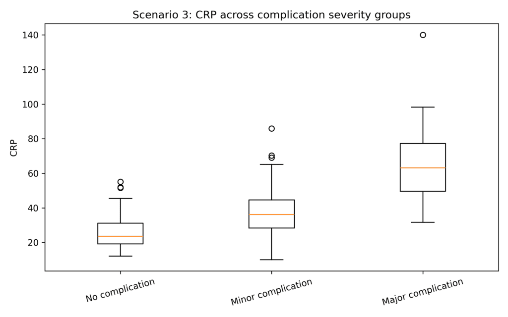
Suppose we want to compare postoperative C-reactive protein levels across three groups of patients:

1. No complication
2. Minor complication
3. Major complication

The question is:

> Do postoperative inflammatory marker levels differ across complication severity groups?

## Why a non-parametric test may be appropriate

Biomarkers such as CRP are notoriously skewed. Some patients show extremely high values because of infection, systemic inflammation, tissue injury, or postoperative complications.

When we have more than two independent groups, the non-parametric analogue of one-way ANOVA is the **Kruskal-Wallis test**.

**Practical assumptions to check**

- Independent groups (each patient contributes to one group only).
- The test detects distributional differences across groups; interpreting it as a comparison of “median differences” is safest only under additional shape assumptions.

## Basic Python example

import numpy as np
import pandas as pd
from scipy.stats import kruskal

np.random.seed(42)

n_no = 45
n_minor = 40
n_major = 35

crp_no = np.random.lognormal(mean=3.2, sigma=0.35, size=n_no)
crp_minor = np.random.lognormal(mean=3.6, sigma=0.40, size=n_minor)
crp_major = np.random.lognormal(mean=4.0, sigma=0.45, size=n_major)

data_crp = pd.DataFrame({
    "group": (
        ["No complication"] * n_no +
        ["Minor complication"] * n_minor +
        ["Major complication"] * n_major
    ),
    "crp": np.concatenate([crp_no, crp_minor, crp_major])
})

stat, p_value = kruskal(
    data_crp.loc[data_crp["group"] == "No complication", "crp"],
    data_crp.loc[data_crp["group"] == "Minor complication", "crp"],
    data_crp.loc[data_crp["group"] == "Major complication", "crp"]
)

print(data_crp.groupby("group")["crp"].median())
print(f"Kruskal-Wallis statistic:{stat:.3f}")
print(f"p-value:{p_value:.4f}")
```
<span class="line"><span style="color: #FF79C6">import</span><span style="color: #F8F8F2"> numpy </span><span style="color: #FF79C6">as</span><span style="color: #F8F8F2"> np</span></span>
<span class="line"><span style="color: #FF79C6">import</span><span style="color: #F8F8F2"> pandas </span><span style="color: #FF79C6">as</span><span style="color: #F8F8F2"> pd</span></span>
<span class="line"><span style="color: #FF79C6">from</span><span style="color: #F8F8F2"> scipy.stats </span><span style="color: #FF79C6">import</span><span style="color: #F8F8F2"> kruskal</span></span>
<span class="line"></span>
<span class="line"><span style="color: #F8F8F2">np.random.seed(</span><span style="color: #BD93F9">42</span><span style="color: #F8F8F2">)</span></span>
<span class="line"></span>
<span class="line"><span style="color: #F8F8F2">n_no </span><span style="color: #FF79C6">=</span><span style="color: #F8F8F2"> </span><span style="color: #BD93F9">45</span></span>
<span class="line"><span style="color: #F8F8F2">n_minor </span><span style="color: #FF79C6">=</span><span style="color: #F8F8F2"> </span><span style="color: #BD93F9">40</span></span>
<span class="line"><span style="color: #F8F8F2">n_major </span><span style="color: #FF79C6">=</span><span style="color: #F8F8F2"> </span><span style="color: #BD93F9">35</span></span>
<span class="line"></span>
<span class="line"><span style="color: #F8F8F2">crp_no </span><span style="color: #FF79C6">=</span><span style="color: #F8F8F2"> np.random.lognormal(</span><span style="color: #FFB86C; font-style: italic">mean</span><span style="color: #FF79C6">=</span><span style="color: #BD93F9">3.2</span><span style="color: #F8F8F2">, </span><span style="color: #FFB86C; font-style: italic">sigma</span><span style="color: #FF79C6">=</span><span style="color: #BD93F9">0.35</span><span style="color: #F8F8F2">, </span><span style="color: #FFB86C; font-style: italic">size</span><span style="color: #FF79C6">=</span><span style="color: #F8F8F2">n_no)</span></span>
<span class="line"><span style="color: #F8F8F2">crp_minor </span><span style="color: #FF79C6">=</span><span style="color: #F8F8F2"> np.random.lognormal(</span><span style="color: #FFB86C; font-style: italic">mean</span><span style="color: #FF79C6">=</span><span style="color: #BD93F9">3.6</span><span style="color: #F8F8F2">, </span><span style="color: #FFB86C; font-style: italic">sigma</span><span style="color: #FF79C6">=</span><span style="color: #BD93F9">0.40</span><span style="color: #F8F8F2">, </span><span style="color: #FFB86C; font-style: italic">size</span><span style="color: #FF79C6">=</span><span style="color: #F8F8F2">n_minor)</span></span>
<span class="line"><span style="color: #F8F8F2">crp_major </span><span style="color: #FF79C6">=</span><span style="color: #F8F8F2"> np.random.lognormal(</span><span style="color: #FFB86C; font-style: italic">mean</span><span style="color: #FF79C6">=</span><span style="color: #BD93F9">4.0</span><span style="color: #F8F8F2">, </span><span style="color: #FFB86C; font-style: italic">sigma</span><span style="color: #FF79C6">=</span><span style="color: #BD93F9">0.45</span><span style="color: #F8F8F2">, </span><span style="color: #FFB86C; font-style: italic">size</span><span style="color: #FF79C6">=</span><span style="color: #F8F8F2">n_major)</span></span>
<span class="line"></span>
<span class="line"><span style="color: #F8F8F2">data_crp </span><span style="color: #FF79C6">=</span><span style="color: #F8F8F2"> pd.DataFrame({</span></span>
<span class="line"><span style="color: #F8F8F2">    </span><span style="color: #E9F284">"</span><span style="color: #F1FA8C">group</span><span style="color: #E9F284">"</span><span style="color: #F8F8F2">: (</span></span>
<span class="line"><span style="color: #F8F8F2">        [</span><span style="color: #E9F284">"</span><span style="color: #F1FA8C">No complication</span><span style="color: #E9F284">"</span><span style="color: #F8F8F2">] </span><span style="color: #FF79C6">*</span><span style="color: #F8F8F2"> n_no </span><span style="color: #FF79C6">+</span></span>
<span class="line"><span style="color: #F8F8F2">        [</span><span style="color: #E9F284">"</span><span style="color: #F1FA8C">Minor complication</span><span style="color: #E9F284">"</span><span style="color: #F8F8F2">] </span><span style="color: #FF79C6">*</span><span style="color: #F8F8F2"> n_minor </span><span style="color: #FF79C6">+</span></span>
<span class="line"><span style="color: #F8F8F2">        [</span><span style="color: #E9F284">"</span><span style="color: #F1FA8C">Major complication</span><span style="color: #E9F284">"</span><span style="color: #F8F8F2">] </span><span style="color: #FF79C6">*</span><span style="color: #F8F8F2"> n_major</span></span>
<span class="line"><span style="color: #F8F8F2">    ),</span></span>
<span class="line"><span style="color: #F8F8F2">    </span><span style="color: #E9F284">"</span><span style="color: #F1FA8C">crp</span><span style="color: #E9F284">"</span><span style="color: #F8F8F2">: np.concatenate([crp_no, crp_minor, crp_major])</span></span>
<span class="line"><span style="color: #F8F8F2">})</span></span>
<span class="line"></span>
<span class="line"><span style="color: #F8F8F2">stat, p_value </span><span style="color: #FF79C6">=</span><span style="color: #F8F8F2"> kruskal(</span></span>
<span class="line"><span style="color: #F8F8F2">    data_crp.loc[data_crp[</span><span style="color: #E9F284">"</span><span style="color: #F1FA8C">group</span><span style="color: #E9F284">"</span><span style="color: #F8F8F2">] </span><span style="color: #FF79C6">==</span><span style="color: #F8F8F2"> </span><span style="color: #E9F284">"</span><span style="color: #F1FA8C">No complication</span><span style="color: #E9F284">"</span><span style="color: #F8F8F2">, </span><span style="color: #E9F284">"</span><span style="color: #F1FA8C">crp</span><span style="color: #E9F284">"</span><span style="color: #F8F8F2">],</span></span>
<span class="line"><span style="color: #F8F8F2">    data_crp.loc[data_crp[</span><span style="color: #E9F284">"</span><span style="color: #F1FA8C">group</span><span style="color: #E9F284">"</span><span style="color: #F8F8F2">] </span><span style="color: #FF79C6">==</span><span style="color: #F8F8F2"> </span><span style="color: #E9F284">"</span><span style="color: #F1FA8C">Minor complication</span><span style="color: #E9F284">"</span><span style="color: #F8F8F2">, </span><span style="color: #E9F284">"</span><span style="color: #F1FA8C">crp</span><span style="color: #E9F284">"</span><span style="color: #F8F8F2">],</span></span>
<span class="line"><span style="color: #F8F8F2">    data_crp.loc[data_crp[</span><span style="color: #E9F284">"</span><span style="color: #F1FA8C">group</span><span style="color: #E9F284">"</span><span style="color: #F8F8F2">] </span><span style="color: #FF79C6">==</span><span style="color: #F8F8F2"> </span><span style="color: #E9F284">"</span><span style="color: #F1FA8C">Major complication</span><span style="color: #E9F284">"</span><span style="color: #F8F8F2">, </span><span style="color: #E9F284">"</span><span style="color: #F1FA8C">crp</span><span style="color: #E9F284">"</span><span style="color: #F8F8F2">]</span></span>
<span class="line"><span style="color: #F8F8F2">)</span></span>
<span class="line"></span>
<span class="line"><span style="color: #8BE9FD">print</span><span style="color: #F8F8F2">(data_crp.groupby(</span><span style="color: #E9F284">"</span><span style="color: #F1FA8C">group</span><span style="color: #E9F284">"</span><span style="color: #F8F8F2">)[</span><span style="color: #E9F284">"</span><span style="color: #F1FA8C">crp</span><span style="color: #E9F284">"</span><span style="color: #F8F8F2">].median())</span></span>
<span class="line"><span style="color: #8BE9FD">print</span><span style="color: #F8F8F2">(</span><span style="color: #FF79C6">f</span><span style="color: #F1FA8C">"Kruskal-Wallis statistic:</span><span style="color: #BD93F9">{</span><span style="color: #F8F8F2">stat</span><span style="color: #FF79C6">:.3f</span><span style="color: #BD93F9">}</span><span style="color: #F1FA8C">"</span><span style="color: #F8F8F2">)</span></span>
<span class="line"><span style="color: #8BE9FD">print</span><span style="color: #F8F8F2">(</span><span style="color: #FF79C6">f</span><span style="color: #F1FA8C">"p-value:</span><span style="color: #BD93F9">{</span><span style="color: #F8F8F2">p_value</span><span style="color: #FF79C6">:.4f</span><span style="color: #BD93F9">}</span><span style="color: #F1FA8C">"</span><span style="color: #F8F8F2">)</span></span>
<span class="line"></span>
```

![Graph of CRP across complication severity groups](https://www.micheledpierri.com/wp-content/uploads/2026/05/scenario_3_crp_boxplot-1024x640.png)

## Interpretation

A significant Kruskal-Wallis test tells us that at least one group tends to differ from the others. It does not, on its own, tell us which groups differ.

When the global test is significant, post-hoc pairwise comparisons may be performed, commonly using Mann-Whitney U tests with correction for multiple comparisons. The plan, however, should be prespecified and reported transparently. Adding tests after seeing the data is a recipe for false-positive findings.

A reasonable reporting sentence:

> CRP levels differed across complication groups according to the Kruskal-Wallis test. Post-hoc pairwise comparisons were then performed with correction for multiple testing.

---

## Scenario 4: Repeated Ordinal Clinical Scores Over Time

## Clinical question

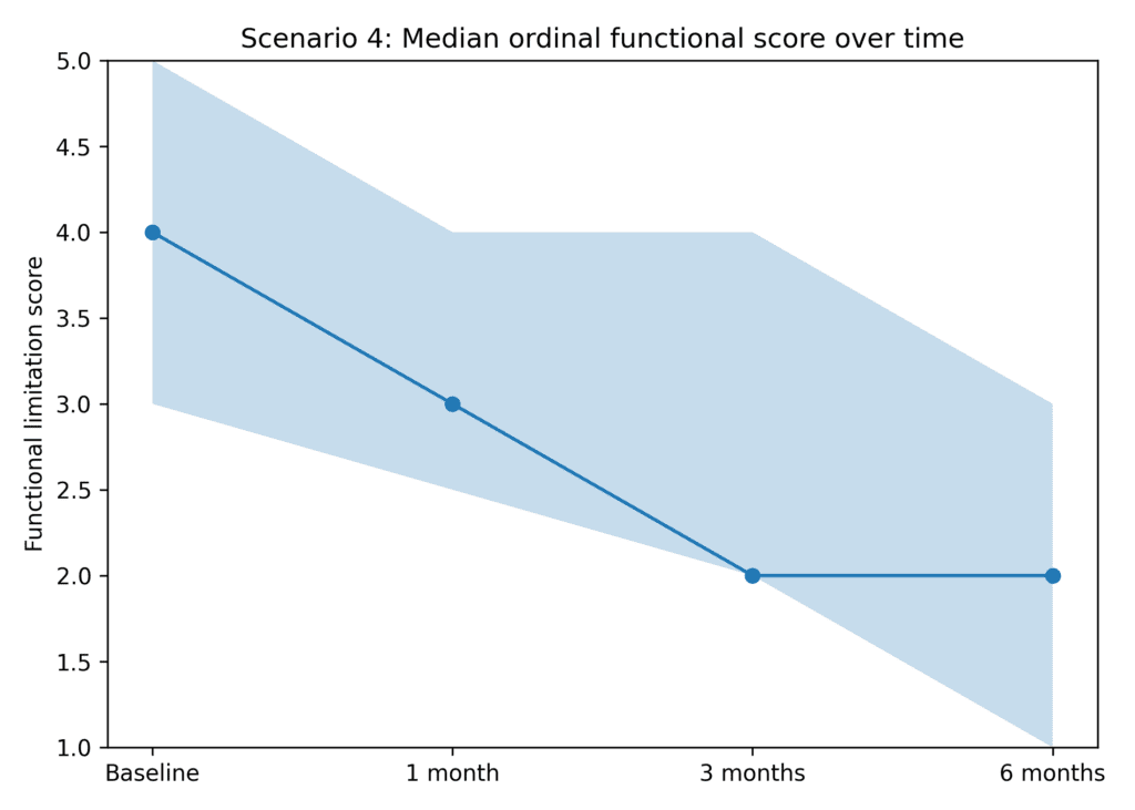
A group of patients is followed after a rehabilitation program. Functional limitation is measured at baseline, 1 month, 3 months, and 6 months using an ordinal score from 1 to 5, where higher values indicate worse functional limitation.

The question is:

> Does functional limitation improve over time?

## Why a non-parametric test may be appropriate

The score is ordinal. The distance between score 1 and score 2 is not necessarily the same as the distance between score 4 and score 5; in fact, in clinical experience, the jump from 4 to 5 often represents a far more substantial functional deterioration. In addition, the same patients are measured repeatedly over time.

The appropriate non-parametric test in this situation is the **Friedman test**, the non-parametric analogue of repeated-measures ANOVA for ranked data.

**Practical assumptions to check**

- Repeated measurements are on the same subjects across time points (complete blocks are ideal).
- The ordinal scale is appropriate for rank-based comparisons. If missingness is substantial, dedicated longitudinal methods may be preferable.

## Basic Python example

import numpy as np
import pandas as pd
from scipy.stats import friedmanchisquare

np.random.seed(42)

n = 35

baseline = np.random.choice([3, 4, 5], size=n, p=[0.25, 0.45, 0.30])
month_1 = np.clip(baseline - np.random.choice([0, 1], size=n, p=[0.45, 0.55]), 1, 5)
month_3 = np.clip(month_1 - np.random.choice([0, 1], size=n, p=[0.40, 0.60]), 1, 5)
month_6 = np.clip(month_3 - np.random.choice([0, 1], size=n, p=[0.55, 0.45]), 1, 5)

data_function = pd.DataFrame({
    "patient_id": range(1, n + 1),
    "baseline": baseline,
    "month_1": month_1,
    "month_3": month_3,
    "month_6": month_6
})

stat, p_value = friedmanchisquare(
    data_function["baseline"],
    data_function["month_1"],
    data_function["month_3"],
    data_function["month_6"]
)

print(data_function.head())
print(f"Friedman statistic:{stat:.3f}")
print(f"p-value:{p_value:.4f}")
```
<span class="line"><span style="color: #FF79C6">import</span><span style="color: #F8F8F2"> numpy </span><span style="color: #FF79C6">as</span><span style="color: #F8F8F2"> np</span></span>
<span class="line"><span style="color: #FF79C6">import</span><span style="color: #F8F8F2"> pandas </span><span style="color: #FF79C6">as</span><span style="color: #F8F8F2"> pd</span></span>
<span class="line"><span style="color: #FF79C6">from</span><span style="color: #F8F8F2"> scipy.stats </span><span style="color: #FF79C6">import</span><span style="color: #F8F8F2"> friedmanchisquare</span></span>
<span class="line"></span>
<span class="line"><span style="color: #F8F8F2">np.random.seed(</span><span style="color: #BD93F9">42</span><span style="color: #F8F8F2">)</span></span>
<span class="line"></span>
<span class="line"><span style="color: #F8F8F2">n </span><span style="color: #FF79C6">=</span><span style="color: #F8F8F2"> </span><span style="color: #BD93F9">35</span></span>
<span class="line"></span>
<span class="line"><span style="color: #F8F8F2">baseline </span><span style="color: #FF79C6">=</span><span style="color: #F8F8F2"> np.random.choice([</span><span style="color: #BD93F9">3</span><span style="color: #F8F8F2">, </span><span style="color: #BD93F9">4</span><span style="color: #F8F8F2">, </span><span style="color: #BD93F9">5</span><span style="color: #F8F8F2">], </span><span style="color: #FFB86C; font-style: italic">size</span><span style="color: #FF79C6">=</span><span style="color: #F8F8F2">n, </span><span style="color: #FFB86C; font-style: italic">p</span><span style="color: #FF79C6">=</span><span style="color: #F8F8F2">[</span><span style="color: #BD93F9">0.25</span><span style="color: #F8F8F2">, </span><span style="color: #BD93F9">0.45</span><span style="color: #F8F8F2">, </span><span style="color: #BD93F9">0.30</span><span style="color: #F8F8F2">])</span></span>
<span class="line"><span style="color: #F8F8F2">month_1 </span><span style="color: #FF79C6">=</span><span style="color: #F8F8F2"> np.clip(baseline </span><span style="color: #FF79C6">-</span><span style="color: #F8F8F2"> np.random.choice([</span><span style="color: #BD93F9">0</span><span style="color: #F8F8F2">, </span><span style="color: #BD93F9">1</span><span style="color: #F8F8F2">], </span><span style="color: #FFB86C; font-style: italic">size</span><span style="color: #FF79C6">=</span><span style="color: #F8F8F2">n, </span><span style="color: #FFB86C; font-style: italic">p</span><span style="color: #FF79C6">=</span><span style="color: #F8F8F2">[</span><span style="color: #BD93F9">0.45</span><span style="color: #F8F8F2">, </span><span style="color: #BD93F9">0.55</span><span style="color: #F8F8F2">]), </span><span style="color: #BD93F9">1</span><span style="color: #F8F8F2">, </span><span style="color: #BD93F9">5</span><span style="color: #F8F8F2">)</span></span>
<span class="line"><span style="color: #F8F8F2">month_3 </span><span style="color: #FF79C6">=</span><span style="color: #F8F8F2"> np.clip(month_1 </span><span style="color: #FF79C6">-</span><span style="color: #F8F8F2"> np.random.choice([</span><span style="color: #BD93F9">0</span><span style="color: #F8F8F2">, </span><span style="color: #BD93F9">1</span><span style="color: #F8F8F2">], </span><span style="color: #FFB86C; font-style: italic">size</span><span style="color: #FF79C6">=</span><span style="color: #F8F8F2">n, </span><span style="color: #FFB86C; font-style: italic">p</span><span style="color: #FF79C6">=</span><span style="color: #F8F8F2">[</span><span style="color: #BD93F9">0.40</span><span style="color: #F8F8F2">, </span><span style="color: #BD93F9">0.60</span><span style="color: #F8F8F2">]), </span><span style="color: #BD93F9">1</span><span style="color: #F8F8F2">, </span><span style="color: #BD93F9">5</span><span style="color: #F8F8F2">)</span></span>
<span class="line"><span style="color: #F8F8F2">month_6 </span><span style="color: #FF79C6">=</span><span style="color: #F8F8F2"> np.clip(month_3 </span><span style="color: #FF79C6">-</span><span style="color: #F8F8F2"> np.random.choice([</span><span style="color: #BD93F9">0</span><span style="color: #F8F8F2">, </span><span style="color: #BD93F9">1</span><span style="color: #F8F8F2">], </span><span style="color: #FFB86C; font-style: italic">size</span><span style="color: #FF79C6">=</span><span style="color: #F8F8F2">n, </span><span style="color: #FFB86C; font-style: italic">p</span><span style="color: #FF79C6">=</span><span style="color: #F8F8F2">[</span><span style="color: #BD93F9">0.55</span><span style="color: #F8F8F2">, </span><span style="color: #BD93F9">0.45</span><span style="color: #F8F8F2">]), </span><span style="color: #BD93F9">1</span><span style="color: #F8F8F2">, </span><span style="color: #BD93F9">5</span><span style="color: #F8F8F2">)</span></span>
<span class="line"></span>
<span class="line"><span style="color: #F8F8F2">data_function </span><span style="color: #FF79C6">=</span><span style="color: #F8F8F2"> pd.DataFrame({</span></span>
<span class="line"><span style="color: #F8F8F2">    </span><span style="color: #E9F284">"</span><span style="color: #F1FA8C">patient_id</span><span style="color: #E9F284">"</span><span style="color: #F8F8F2">: </span><span style="color: #8BE9FD">range</span><span style="color: #F8F8F2">(</span><span style="color: #BD93F9">1</span><span style="color: #F8F8F2">, n </span><span style="color: #FF79C6">+</span><span style="color: #F8F8F2"> </span><span style="color: #BD93F9">1</span><span style="color: #F8F8F2">),</span></span>
<span class="line"><span style="color: #F8F8F2">    </span><span style="color: #E9F284">"</span><span style="color: #F1FA8C">baseline</span><span style="color: #E9F284">"</span><span style="color: #F8F8F2">: baseline,</span></span>
<span class="line"><span style="color: #F8F8F2">    </span><span style="color: #E9F284">"</span><span style="color: #F1FA8C">month_1</span><span style="color: #E9F284">"</span><span style="color: #F8F8F2">: month_1,</span></span>
<span class="line"><span style="color: #F8F8F2">    </span><span style="color: #E9F284">"</span><span style="color: #F1FA8C">month_3</span><span style="color: #E9F284">"</span><span style="color: #F8F8F2">: month_3,</span></span>
<span class="line"><span style="color: #F8F8F2">    </span><span style="color: #E9F284">"</span><span style="color: #F1FA8C">month_6</span><span style="color: #E9F284">"</span><span style="color: #F8F8F2">: month_6</span></span>
<span class="line"><span style="color: #F8F8F2">})</span></span>
<span class="line"></span>
<span class="line"><span style="color: #F8F8F2">stat, p_value </span><span style="color: #FF79C6">=</span><span style="color: #F8F8F2"> friedmanchisquare(</span></span>
<span class="line"><span style="color: #F8F8F2">    data_function[</span><span style="color: #E9F284">"</span><span style="color: #F1FA8C">baseline</span><span style="color: #E9F284">"</span><span style="color: #F8F8F2">],</span></span>
<span class="line"><span style="color: #F8F8F2">    data_function[</span><span style="color: #E9F284">"</span><span style="color: #F1FA8C">month_1</span><span style="color: #E9F284">"</span><span style="color: #F8F8F2">],</span></span>
<span class="line"><span style="color: #F8F8F2">    data_function[</span><span style="color: #E9F284">"</span><span style="color: #F1FA8C">month_3</span><span style="color: #E9F284">"</span><span style="color: #F8F8F2">],</span></span>
<span class="line"><span style="color: #F8F8F2">    data_function[</span><span style="color: #E9F284">"</span><span style="color: #F1FA8C">month_6</span><span style="color: #E9F284">"</span><span style="color: #F8F8F2">]</span></span>
<span class="line"><span style="color: #F8F8F2">)</span></span>
<span class="line"></span>
<span class="line"><span style="color: #8BE9FD">print</span><span style="color: #F8F8F2">(data_function.head())</span></span>
<span class="line"><span style="color: #8BE9FD">print</span><span style="color: #F8F8F2">(</span><span style="color: #FF79C6">f</span><span style="color: #F1FA8C">"Friedman statistic:</span><span style="color: #BD93F9">{</span><span style="color: #F8F8F2">stat</span><span style="color: #FF79C6">:.3f</span><span style="color: #BD93F9">}</span><span style="color: #F1FA8C">"</span><span style="color: #F8F8F2">)</span></span>
<span class="line"><span style="color: #8BE9FD">print</span><span style="color: #F8F8F2">(</span><span style="color: #FF79C6">f</span><span style="color: #F1FA8C">"p-value:</span><span style="color: #BD93F9">{</span><span style="color: #F8F8F2">p_value</span><span style="color: #FF79C6">:.4f</span><span style="color: #BD93F9">}</span><span style="color: #F1FA8C">"</span><span style="color: #F8F8F2">)</span></span>
<span class="line"></span>
```

![Median ordinal functional score over time](https://www.micheledpierri.com/wp-content/uploads/2026/05/scenario_4_functional_score_over_time-1024x731.png)

## Interpretation

A significant Friedman test suggests that the repeated measurements are not all drawn from the same distribution. In our example, it would support the presence of a change in functional limitation over time.

As with Kruskal-Wallis, the global test does not identify which time points differ. When needed, post-hoc paired comparisons can be performed with appropriate correction.

A reasonable reporting sentence:

> Functional limitation improved over time. The overall change across follow-up visits was significant according to the Friedman test.

---

# Practical Decision Table


| Clinical scenario | Data structure | Typical variable | Parametric test | Non-parametric test |
| --- | --- | --- | --- | --- |
| Pain before and after therapy | Paired observations | VAS score | Paired t-test | Wilcoxon signed-rank test |
| Length of stay in two groups | Two independent groups | Days of hospitalization | Independent t-test | Mann-Whitney U test |
| Biomarker across severity groups | More than two independent groups | CRP, ferritin, D-dimer | One-way ANOVA | Kruskal-Wallis test |
| Ordinal score over time | Repeated measures | Functional score, NYHA-like score | Repeated-measures ANOVA | Friedman test |

---

# Common Mistakes in Medical Papers

## 1. Using non-parametric tests automatically after a significant normality test

Normality tests can be overly sensitive in large samples and underpowered in small samples. The decision should also rest on histograms, Q-Q plots, clinical plausibility, outliers, and the actual scale of measurement. Mechanical reliance on a single test is rarely a good idea.

## 2. Saying that Mann-Whitney always compares medians

This is a common oversimplification. When the two distributions have a similar shape, the Mann-Whitney U test can be interpreted as a test of location shift. When the distributions differ in shape or spread, the interpretation is broader: one group tends to have larger or smaller values than the other.

## 3. Reporting mean and standard deviation for markedly skewed variables

For strongly skewed variables, median and interquartile range are usually more clinically informative.

## 4. Reporting only p-values

A p-value does not quantify clinical relevance. Whenever possible, the report should include effect sizes, median differences, confidence intervals, and clinically interpretable summaries.

## 5. Ignoring multiple comparisons

After a significant Kruskal-Wallis or Friedman test, post-hoc comparisons must account for multiplicity. Otherwise, the probability of false-positive findings rises quickly.

## 6. Confusing statistical significance with clinical importance

A statistically significant reduction in pain score may still be clinically irrelevant when the magnitude is small. Conversely, a clinically relevant difference can easily fail to reach statistical significance in a small pilot study.

---

# How to Report Non-Parametric Analyses

A concise reporting style could be:

> Continuous skewed variables were summarized as median and interquartile range. Between-group comparisons were performed using the Mann-Whitney U test for two independent groups and the Kruskal-Wallis test for more than two independent groups. Paired before-after comparisons were performed using the Wilcoxon signed-rank test. Repeated ordinal measurements were analyzed using the Friedman test. A two-sided p-value < 0.05 was considered statistically significant.

For a more complete report, effect sizes and confidence intervals should be added where possible. Practical options include:

- Wilcoxon signed-rank: rank-biserial correlation or an r-type effect size (when available).
- Mann-Whitney: rank-biserial correlation or Cliff’s delta.
- Kruskal-Wallis: epsilon-squared (or a similar rank-based η²) to quantify the global effect.
- Friedman: Kendall’s W as an overall effect size.

---

# Conclusion

Non-parametric statistics are particularly useful in medicine, where clinical data are routinely skewed, ordinal, bounded, or affected by outliers. These methods are not a fallback for weak data analysis. In many cases they represent the most appropriate way to analyze real-world clinical variables.

The practical message is straightforward:

> Choose the test according to the clinical question, the study design, and the structure of the variable, not only according to a mechanical normality test.

In clinical research the goal is not to deploy the most sophisticated method available. The goal is to use a method that respects the data and produces an interpretation that is clinically meaningful.

---

# Suggested References

Hollander M, Wolfe DA, Chicken E. _Nonparametric Statistical Methods_. Wiley.

Altman DG. _Practical Statistics for Medical Research_. Chapman & Hall/CRC.

Bland M. _An Introduction to Medical Statistics_. Oxford University Press.

Conover WJ. _Practical Nonparametric Statistics_. Wiley.

---

See also on this site: [Nonparametric statistics](https://www.micheledpierri.com/wp-content/uploads/wp-mfa-exports/page/nonparametric-statistics.md)