---
title: Outliers
date: 2024-09-26T19:44:55Z
modified: 2026-07-04T08:39:38Z
permalink: "https://www.micheledpierri.com/data-analysis/outliers/"
type: page
status: publish
excerpt: ""
wpid: 520
featured_image: "https://www.micheledpierri.com/wp-content/uploads/2026/07/d_a_outliers_.png"
featured_image_alt: Man observes glowing constellations through a brass telescope in a dim early 20th-century hospital ward.
timestamp: 2026-07-04T08:39:38Z
tags: []
---

Imagine a database with a column reporting subjects’ heights. The values range from 150 cm to 200 cm for most subjects. However, there’s one case with a reported height of 250 cm. This value, being both improbable and significantly deviating from the others, is an outlier.

An outlier is an observation that significantly deviates from expected values in a data distribution and may stem from a different mechanism than most other data points.

Identifying and managing outliers is crucial in data cleaning before Exploratory Data Analysis (EDA). These anomalies can distort statistics and complicate interpretation.

In predictive models and machine learning applications, outliers can disproportionately influence the model, skewing results—particularly in linear regression.

## Identifying Outliers

### Identification based on interquartile range

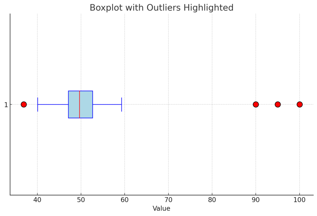
In statistical analysis, we use Q1 to represent the first quartile (25th percentile) and Q3 for the third quartile (75th percentile). The **interquartile range (IQR)** is the difference between Q3 and Q1. An outlier is defined as any value that falls below Q1 – 1.5 × IQR or above Q3 + 1.5 × IQR.

This method is commonly used to identify outliers in box-plot graphs.

Outlier = < Q1 – 1.5 × IQR or value > Q3 + 1.5 × IQR

### Identification based on Z-score

The **Z-Score** measures how far a data point is from the mean, expressed in standard deviations. A value with a Z-Score greater than 3 or less than -3 is typically considered an outlier.

![z = \frac{x - \mu}{\sigma}](https://www.micheledpierri.com/wp-content/ql-cache/quicklatex.com-b0d286cf1959313f0e16d9e62430f842_l3.svg "Rendered by QuickLaTeX.com")

### Mahalanobis distance

The **Mahalanobis distance** is used in multivariate contexts to identify outliers. It measures the distance of a point from an average distribution, taking into account the correlation between variables. This method is particularly useful when data points are not independent of each other. If a point’s Mahalanobis distance is significantly larger than that of other points, it is considered an outlier.

### Density-Based Spatial Clustering of Applications with Noise (DBSCAN)

The **DBSCAN** algorithm effectively identifies outliers in multivariate data. It classifies a point as an outlier when it’s found in a low-density region—essentially, when it’s “isolated” from other data points.

The boxplot chart is the most effective visual tool for evaluating outliers. In this graph, outliers—typically calculated using the interquartile range method—appear beyond the whiskers.
![Boxplot with outliers highlighted](https://www.micheledpierri.com/wp-content/uploads/2024/09/outliers2-1024x696.png)

## Interpreting outliers

Outliers in a dataset can arise from several sources:

1. Errors: These may stem from incorrect data entry, faulty measurements, sensor malfunctions, or improper calibration.
2. Genuine rare occurrences: These reflect unusual but natural phenomena, such as rare genetic mutations, extreme weather events, or financial market crashes.
3. Sampling errors: Non-representative sampling can lead to outliers that don’t accurately reflect the population. For instance, when gathering height data for adults, accidentally including children in the sample would produce outliers.

## Managing Outliers

The simplest way to manage outliers is to delete them, but this approach isn’t always appropriate.

Consider outlier elimination when:

1. There are obvious measurement or input errors
2. They come from non-representative samples
3. They significantly distort the model (for instance, linear regression is particularly sensitive)
4. They’re irrelevant to the analysis at hand

On the other hand, reasons to retain outliers include:

1. The data represents real, albeit rare, important phenomena
2. They’re integral to the system under study
3. They might indicate discoveries or previously unknown phenomena
4. They belong to an inherently asymmetric distribution
5. You’re using a robust analysis method insensitive to outliers (such as Random Forest)

In conclusion, manage outliers on a case-by-case basis. Remove those caused by errors, but keep those that may represent real phenomena and are thus part of the data’s natural distribution.

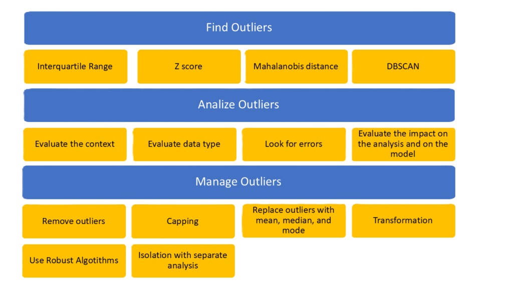
If we choose to retain outliers rather than delete them, several management strategies are available:

1. Capping: Limiting the maximum or minimum values to acceptable thresholds
2. Replacement: Substituting outliers with the mean or median of the dataset
3. Transformation: Applying logarithmic or quadratic functions to the data
4. Robust regression: Using models that are less sensitive to outliers
![Outliers management](https://www.micheledpierri.com/wp-content/uploads/2024/09/Outlier-1024x576.png)

## Python and Outliers

Python offers numerous libraries for efficiently identifying and managing outliers in datasets.

Pandas offers a method to identify outliers using the interquartile range, utilizing its descriptive statistics functions:

import pandas as pd

# Calculation of quantiles
Q1 = df['column'].quantile(0.25)
Q3 = df['column'].quantile(0.75)
IQR = Q3 - Q1

# Identification of outliers
outliers = df[(df['column'] < (Q1 - 1.5 * IQR)) | (df['column'] > (Q3 + 1.5 * IQR))]

```
<span class="line"><span style="color: #FF79C6">import</span><span style="color: #F8F8F2"> pandas </span><span style="color: #FF79C6">as</span><span style="color: #F8F8F2"> pd</span></span>
<span class="line"></span>
<span class="line"><span style="color: #6272A4"># Calculation of quantiles</span></span>
<span class="line"><span style="color: #F8F8F2">Q1 </span><span style="color: #FF79C6">=</span><span style="color: #F8F8F2"> df[</span><span style="color: #E9F284">'</span><span style="color: #F1FA8C">column</span><span style="color: #E9F284">'</span><span style="color: #F8F8F2">].quantile(</span><span style="color: #BD93F9">0.25</span><span style="color: #F8F8F2">)</span></span>
<span class="line"><span style="color: #F8F8F2">Q3 </span><span style="color: #FF79C6">=</span><span style="color: #F8F8F2"> df[</span><span style="color: #E9F284">'</span><span style="color: #F1FA8C">column</span><span style="color: #E9F284">'</span><span style="color: #F8F8F2">].quantile(</span><span style="color: #BD93F9">0.75</span><span style="color: #F8F8F2">)</span></span>
<span class="line"><span style="color: #BD93F9">IQR</span><span style="color: #F8F8F2"> </span><span style="color: #FF79C6">=</span><span style="color: #F8F8F2"> Q3 </span><span style="color: #FF79C6">-</span><span style="color: #F8F8F2"> Q1</span></span>
<span class="line"></span>
<span class="line"><span style="color: #6272A4"># Identification of outliers</span></span>
<span class="line"><span style="color: #F8F8F2">outliers </span><span style="color: #FF79C6">=</span><span style="color: #F8F8F2"> df[(df[</span><span style="color: #E9F284">'</span><span style="color: #F1FA8C">column</span><span style="color: #E9F284">'</span><span style="color: #F8F8F2">] </span><span style="color: #FF79C6"><</span><span style="color: #F8F8F2"> (Q1 </span><span style="color: #FF79C6">-</span><span style="color: #F8F8F2"> </span><span style="color: #BD93F9">1.5</span><span style="color: #F8F8F2"> </span><span style="color: #FF79C6">*</span><span style="color: #F8F8F2"> </span><span style="color: #BD93F9">IQR</span><span style="color: #F8F8F2">)) </span><span style="color: #FF79C6">|</span><span style="color: #F8F8F2"> (df[</span><span style="color: #E9F284">'</span><span style="color: #F1FA8C">column</span><span style="color: #E9F284">'</span><span style="color: #F8F8F2">] </span><span style="color: #FF79C6">></span><span style="color: #F8F8F2"> (Q3 </span><span style="color: #FF79C6">+</span><span style="color: #F8F8F2"> </span><span style="color: #BD93F9">1.5</span><span style="color: #F8F8F2"> </span><span style="color: #FF79C6">*</span><span style="color: #F8F8F2"> </span><span style="color: #BD93F9">IQR</span><span style="color: #F8F8F2">))]</span></span>
<span class="line"></span>
```

The zscore method from scipy calculates the z-score, which identifies outliers as values greater than 3 or less than -3.

from scipy import stats

df['z_score'] = stats.zscore(df['column'])
outliers = df[(df['z_score'] > 3) | (df['z_score'] < -3)]

```
<span class="line"><span style="color: #FF79C6">from</span><span style="color: #F8F8F2"> scipy </span><span style="color: #FF79C6">import</span><span style="color: #F8F8F2"> stats</span></span>
<span class="line"></span>
<span class="line"><span style="color: #F8F8F2">df[</span><span style="color: #E9F284">'</span><span style="color: #F1FA8C">z_score</span><span style="color: #E9F284">'</span><span style="color: #F8F8F2">] </span><span style="color: #FF79C6">=</span><span style="color: #F8F8F2"> stats.zscore(df[</span><span style="color: #E9F284">'</span><span style="color: #F1FA8C">column</span><span style="color: #E9F284">'</span><span style="color: #F8F8F2">])</span></span>
<span class="line"><span style="color: #F8F8F2">outliers </span><span style="color: #FF79C6">=</span><span style="color: #F8F8F2"> df[(df[</span><span style="color: #E9F284">'</span><span style="color: #F1FA8C">z_score</span><span style="color: #E9F284">'</span><span style="color: #F8F8F2">] </span><span style="color: #FF79C6">></span><span style="color: #F8F8F2"> </span><span style="color: #BD93F9">3</span><span style="color: #F8F8F2">) </span><span style="color: #FF79C6">|</span><span style="color: #F8F8F2"> (df[</span><span style="color: #E9F284">'</span><span style="color: #F1FA8C">z_score</span><span style="color: #E9F284">'</span><span style="color: #F8F8F2">] </span><span style="color: #FF79C6"><</span><span style="color: #F8F8F2"> </span><span style="color: #FF79C6">-</span><span style="color: #BD93F9">3</span><span style="color: #F8F8F2">)]</span></span>
<span class="line"></span>
```

For graphical visualization, seaborn can be used to create boxplots:

import seaborn as sns

sns.boxplot(x=df['column'])

```
<span class="line"><span style="color: #FF79C6">import</span><span style="color: #F8F8F2"> seaborn </span><span style="color: #FF79C6">as</span><span style="color: #F8F8F2"> sns</span></span>
<span class="line"></span>
<span class="line"><span style="color: #F8F8F2">sns.boxplot(</span><span style="color: #FFB86C; font-style: italic">x</span><span style="color: #FF79C6">=</span><span style="color: #F8F8F2">df[</span><span style="color: #E9F284">'</span><span style="color: #F1FA8C">column</span><span style="color: #E9F284">'</span><span style="color: #F8F8F2">])</span></span>
<span class="line"></span>
```

Pandas can be used to efficiently remove outliers:

df_cleaned = df[(df['column'] >= Q1 - 1.5 * IQR) & (df['column'] <= Q3 + 1.5 * IQR)]

```
<span class="line"><span style="color: #F8F8F2">df_cleaned </span><span style="color: #FF79C6">=</span><span style="color: #F8F8F2"> df[(df[</span><span style="color: #E9F284">'</span><span style="color: #F1FA8C">column</span><span style="color: #E9F284">'</span><span style="color: #F8F8F2">] </span><span style="color: #FF79C6">>=</span><span style="color: #F8F8F2"> Q1 </span><span style="color: #FF79C6">-</span><span style="color: #F8F8F2"> </span><span style="color: #BD93F9">1.5</span><span style="color: #F8F8F2"> </span><span style="color: #FF79C6">*</span><span style="color: #F8F8F2"> </span><span style="color: #BD93F9">IQR</span><span style="color: #F8F8F2">) </span><span style="color: #FF79C6">&</span><span style="color: #F8F8F2"> (df[</span><span style="color: #E9F284">'</span><span style="color: #F1FA8C">column</span><span style="color: #E9F284">'</span><span style="color: #F8F8F2">] </span><span style="color: #FF79C6"><=</span><span style="color: #F8F8F2"> Q3 </span><span style="color: #FF79C6">+</span><span style="color: #F8F8F2"> </span><span style="color: #BD93F9">1.5</span><span style="color: #F8F8F2"> </span><span style="color: #FF79C6">*</span><span style="color: #F8F8F2"> </span><span style="color: #BD93F9">IQR</span><span style="color: #F8F8F2">)]</span></span>
<span class="line"></span>
```

Capping or replacing values with the mean and median can be accomplished using pandas and numpy:

# Limit values to the 1st and 99th percentiles
lower_limit = df['column'].quantile(0.01)
upper_limit = df['column'].quantile(0.99)
df['column'] = np.where(df['column'] < lower_limit, lower_limit, df['column'])
df['column'] = np.where(df['column'] > upper_limit, upper_limit, df['column'])

# Replaces with median
median = df['column'].median()
df['column'] = np.where(df['column'] > upper_limit, median, df['column'])

```
<span class="line"><span style="color: #6272A4"># Limit values to the 1st and 99th percentiles</span></span>
<span class="line"><span style="color: #F8F8F2">lower_limit </span><span style="color: #FF79C6">=</span><span style="color: #F8F8F2"> df[</span><span style="color: #E9F284">'</span><span style="color: #F1FA8C">column</span><span style="color: #E9F284">'</span><span style="color: #F8F8F2">].quantile(</span><span style="color: #BD93F9">0.01</span><span style="color: #F8F8F2">)</span></span>
<span class="line"><span style="color: #F8F8F2">upper_limit </span><span style="color: #FF79C6">=</span><span style="color: #F8F8F2"> df[</span><span style="color: #E9F284">'</span><span style="color: #F1FA8C">column</span><span style="color: #E9F284">'</span><span style="color: #F8F8F2">].quantile(</span><span style="color: #BD93F9">0.99</span><span style="color: #F8F8F2">)</span></span>
<span class="line"><span style="color: #F8F8F2">df[</span><span style="color: #E9F284">'</span><span style="color: #F1FA8C">column</span><span style="color: #E9F284">'</span><span style="color: #F8F8F2">] </span><span style="color: #FF79C6">=</span><span style="color: #F8F8F2"> np.where(df[</span><span style="color: #E9F284">'</span><span style="color: #F1FA8C">column</span><span style="color: #E9F284">'</span><span style="color: #F8F8F2">] </span><span style="color: #FF79C6"><</span><span style="color: #F8F8F2"> lower_limit, lower_limit, df[</span><span style="color: #E9F284">'</span><span style="color: #F1FA8C">column</span><span style="color: #E9F284">'</span><span style="color: #F8F8F2">])</span></span>
<span class="line"><span style="color: #F8F8F2">df[</span><span style="color: #E9F284">'</span><span style="color: #F1FA8C">column</span><span style="color: #E9F284">'</span><span style="color: #F8F8F2">] </span><span style="color: #FF79C6">=</span><span style="color: #F8F8F2"> np.where(df[</span><span style="color: #E9F284">'</span><span style="color: #F1FA8C">column</span><span style="color: #E9F284">'</span><span style="color: #F8F8F2">] </span><span style="color: #FF79C6">></span><span style="color: #F8F8F2"> upper_limit, upper_limit, df[</span><span style="color: #E9F284">'</span><span style="color: #F1FA8C">column</span><span style="color: #E9F284">'</span><span style="color: #F8F8F2">])</span></span>
<span class="line"></span>
<span class="line"><span style="color: #6272A4"># Replaces with median</span></span>
<span class="line"><span style="color: #F8F8F2">median </span><span style="color: #FF79C6">=</span><span style="color: #F8F8F2"> df[</span><span style="color: #E9F284">'</span><span style="color: #F1FA8C">column</span><span style="color: #E9F284">'</span><span style="color: #F8F8F2">].median()</span></span>
<span class="line"><span style="color: #F8F8F2">df[</span><span style="color: #E9F284">'</span><span style="color: #F1FA8C">column</span><span style="color: #E9F284">'</span><span style="color: #F8F8F2">] </span><span style="color: #FF79C6">=</span><span style="color: #F8F8F2"> np.where(df[</span><span style="color: #E9F284">'</span><span style="color: #F1FA8C">column</span><span style="color: #E9F284">'</span><span style="color: #F8F8F2">] </span><span style="color: #FF79C6">></span><span style="color: #F8F8F2"> upper_limit, median, df[</span><span style="color: #E9F284">'</span><span style="color: #F1FA8C">column</span><span style="color: #E9F284">'</span><span style="color: #F8F8F2">])</span></span>
<span class="line"></span>
```

## SPSS and Outliers

SPSS provides several tools for identifying outliers:

- **Boxplot**: A common visual tool in SPSS for spotting outliers. These appear as points beyond the boxplot’s “whiskers.” 
    - Navigate to `Graphs > Chart Builder`, choose `Boxplot`, and select your variable of interest.
- **Descriptive Statistics**: Use `Analyze > Descriptive Statistics > Descriptives` to compute Z-scores. Values exceeding ±3 typically signify outliers.
- **Explore Command**: Access `Analyze - Descriptive Statistics > Explore` for a comprehensive table. This includes percentiles, interquartile range (IQR), and visualizations like boxplots and stem-and-leaf plots—all helpful for outlier identification.

Once outliers have been identified, SPSS offers several options for managing them:

**Removal of Outliers**: You can simply filter or remove outliers from your data. Use `Data > Select Cases` and set a condition based on a range of acceptable values (for example, remove all cases with Z-scores beyond ±3).

**Imputation**:

**Replace with Mean or Median**: You can replace outliers with the mean or median of non-outlier observations. This can be done manually with `Transform > Compute Variable`, where you can create a new variable replacing outlier values with the mean or median.

**Capping**:

SPSS doesn’t have a specific command for capping, but it can be done manually. It involves replacing outliers with the maximum/minimum acceptable value (e.g., the 5th and 95th percentiles). You can create a new variable using `Transform > Compute Variable` and setting conditions to replace extreme values.

**Transformations**:

**Log Transformation, Square Root Transformation**: Logarithmic or square root transformations can be applied to reduce the impact of outliers on subsequent analyses. Use `Transform > Compute Variable` to create a new transformed variable.

**Model-Based Methods**:

**Robust Regression**: SPSS also offers robust regression models such as `Robust Regression` that can be used to minimize the influence of outliers. This option is available through the regression menus in `Analyze > Regression > Linear` and choosing robust regression methods under “Method”.