---
title: Linear Regression
date: 2025-03-29T15:19:22Z
modified: 2026-07-28T07:50:30Z
permalink: "https://www.micheledpierri.com/machine-learning/linear-regression-in-machine-learning/"
type: page
status: publish
excerpt: ""
wpid: 1197
featured_image: "https://www.micheledpierri.com/wp-content/uploads/2026/07/ml_linear_regression_.png"
featured_image_alt: Young boy gazing at towering crates of fruit and vegetables outside a rustic village market in warm golden light.
timestamp: 2026-07-28T07:50:30Z
tags: []
---
Note: additional posts about linear regression can be found elsewhere on this site, offering a [more statistical perspective](https://www.micheledpierri.com/wp-content/uploads/wp-mfa-exports/page/linear-regression-in-statistics.md).
## Introduction to Linear Regression
Regression models are supervised learning algorithms that analyze how one or more input variables affect a continuous dependent variable (output).
Regression models come in several distinct types: linear regression is one of the most widely used and straightforward machine learning algorithms. It finds a linear relationship between a continuous dependent variable and one independent variable (simple regression) or multiple independent variables (multiple regression).
A classic example is using years of experience (the independent variable) to predict salary level (the dependent variable).
In medical applications (such as predicting length of stay, disease progression, or blood levels), a regression model must meet three key requirements:
- **does not present systematic bias** (for example, underestimating severity in critical patients),
- **has good predictive power on new data** (generalization),
- **is interpretable**, including at the diagnostic level (such as residual analysis).
## Mathematical Foundations of Linear Regression
The formula for simple linear regression is:

where x and y represent the independent and dependent variables respectively, β₀ is the intercept, and β₁ is the slope coefficient (indicating how much y changes when x changes). ε represents the residual error.
The multiple linear regression formula includes several independent variables, each with its coefficient:

Each coefficient represents the impact of its corresponding variable on y while keeping all other variables constant.
### Summary of Definitions
| Term | Definition | Example |
| --- | --- | --- |
| Intercept (_β_₀) | Value of _y_ when all _x_ values are zero. | Initial salary with zero experience. |
| Slope (_β_₁) | Change in _y_ for each unit increase in _x_. | Salary increase for each year of experience. |
| Coefficients (_β_ᵢ) | Impact of each variable_xᵢ_on_y_, holding other factors constant. | Impact of education level on salary. |
| Residual Error (_ε_) | Difference between observed _y_ and predicted _y_ (_ŷ_). | Prediction error for each observation. |
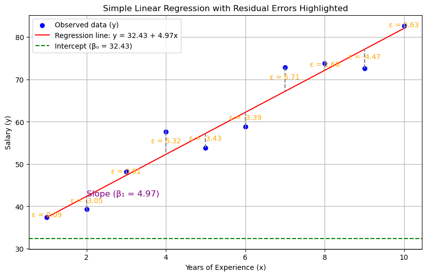
Residuals represent the difference between observed values and model predictions:

where:
 = residual for observation i

= observed values (actual values)

= predicted values
Analyzing residuals serves two crucial purposes: assessing model quality through their magnitude and verifying that the regression assumptions are satisfied.
Although linear regression originated in statistics, it functions as a supervised machine learning algorithm: During the training phase, the model learns the coefficients by minimizing the error, then generates predictions in the form of continuous variables.
## When to use linear regression
Linear regression requires a continuous dependent variable, as categorical variables need different algorithms. The model performs best with linear relationships between variables. For non-linear relationships, it is necessary to use polynomial regression or neural networks instead.
One key advantage of linear regression is its interpretability, as the beta coefficients clearly show how each independent variable affects the dependent variable.
The model performs well with small and medium-sized datasets, needing relatively few data points for training. However, the number of independent variables (p) should not exceed the number of cases (n). When p>n, alternative regression methods are more appropriate.
The model also assumes no multicollinearity between variables. If variables are highly correlated, consider using Ridge or Lasso regression instead.
## When Not to Use Linear Regression
Non-linear relationships between variables
High-dimensional datasets where predictors exceed observations (p≫n)
Strong correlation between predictor variables (multicollinearity)
When predicting categorical outcomes
When key statistical assumptions are violated
When higher accuracy requires more sophisticated models
## Linear Regression Assumptions
Linear regression requires these essential conditions to be valid:
A linear relationship between independent (X) and dependent (y) variables
Independent residual errors with no correlation between them
Homoscedasticity—constant variance of errors across all observations
Normally distributed residual errors
## Linear Regression in Python
To demonstrate linear regression in Python, we’ll use the diabetes database from scikit-learn.
This dataset contains real-world data that predicts one-year disease progression using laboratory parameters.
The dataset includes 442 patient observations, with 10 parameters recorded for each patient (including age, sex, body mass index, blood pressure, cholesterol, and others).
The continuous target variable measures disease progression at the one-year mark.
The dataset’s values are already [normalized](https://www.micheledpierri.com/wp-content/uploads/wp-mfa-exports/page/normalization-standardization-and-scalers.md), ranging from 0 to 1.
from sklearn.datasets import load_diabetes
import pandas as pd
import numpy as np
# Loading dataset
data = load_diabetes()
X = pd.DataFrame(data.data, columns=data.feature_names)
y = pd.Series(data.target, name='target')
# Check
print(X.head())
print(y.head())```
from sklearn.datasets import load_diabetes
import pandas as pd
import numpy as np
# Loading dataset
data = load_diabetes()
X = pd.DataFrame(data.data, columns=data.feature_names)
y = pd.Series(data.target, name='target')
# Check
print(X.head())
print(y.head())
```
### Simple Linear Regression Example
To demonstrate simple linear regression, we’ll focus on a single feature: body mass index. This will allow us to analyze the linear relationship between body mass index and disease progression.
from sklearn.linear_model import LinearRegression
from sklearn.model_selection import train_test_split
from sklearn.metrics import mean_squared_error, r2_score
import matplotlib.pyplot as plt
# Select BMI as the single predictor variable
X_bmi = X[['bmi']]
y = y # Target variable
# Split data into training and test sets
X_train, X_test, y_train, y_test = train_test_split(X_bmi, y, test_size=0.2, random_state=42)
# Create and train the model
model_simple = LinearRegression()
model_simple.fit(X_train, y_train)
# Make predictions on test set
y_pred = model_simple.predict(X_test)
# Calculate model performance metrics
print("Coefficient:", model_simple.coef_[0])
print("Intercept:", model_simple.intercept_)
print("MSE:", mean_squared_error(y_test, y_pred))
print("R² score:", r2_score(y_test, y_pred))
# Create visualization
plt.scatter(X_test, y_test, color='blue', label='True values')
plt.plot(X_test, y_pred, color='red', linewidth=2, label='Regression line')
plt.xlabel('BMI')
plt.ylabel('Disease progression')
plt.legend()
plt.title('Simple Linear Regression')
plt.show()```
from sklearn.linear_model import LinearRegression
from sklearn.model_selection import train_test_split
from sklearn.metrics import mean_squared_error, r2_score
import matplotlib.pyplot as plt
# Select BMI as the single predictor variable
X_bmi = X[['bmi']]
y = y # Target variable
# Split data into training and test sets
X_train, X_test, y_train, y_test = train_test_split(X_bmi, y, test_size=0.2, random_state=42)
# Create and train the model
model_simple = LinearRegression()
model_simple.fit(X_train, y_train)
# Make predictions on test set
y_pred = model_simple.predict(X_test)
# Calculate model performance metrics
print("Coefficient:", model_simple.coef_[0])
print("Intercept:", model_simple.intercept_)
print("MSE:", mean_squared_error(y_test, y_pred))
print("R² score:", r2_score(y_test, y_pred))
# Create visualization
plt.scatter(X_test, y_test, color='blue', label='True values')
plt.plot(X_test, y_pred, color='red', linewidth=2, label='Regression line')
plt.xlabel('BMI')
plt.ylabel('Disease progression')
plt.legend()
plt.title('Simple Linear Regression')
plt.show()
```
#### Results:
- Coefficient: 998.5776891375593
- Intercept: 152.00335421448167
- MSE: 4061.8259284949268
- R² score: 0.23335039815872138
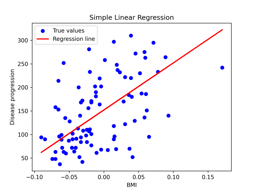
In this example:
The coefficient of 998.58 indicates that a 1-unit increase in standardized BMI corresponds to a 998-unit increase in one-year disease progression.
The intercept of 152 represents the disease progression value when BMI is at its standardized mean (zero).
MSE (mean squared error) measures the average squared difference between predicted and observed values.
The R² value of 0.23 indicates that BMI alone explains only 23% of the variability in disease progression—a relatively modest predictive power.
These results indicate that while BMI has a significant association with diabetic disease progression, it alone cannot accurately predict the outcome. A more comprehensive model incorporating all available variables would provide better predictive power.
### Multiple Linear Regression Example
Next, we’ll build a model incorporating all features from the diabetes dataset.
# All features
X_all = X
y = y
# Split
X_train, X_test, y_train, y_test = train_test_split(X_all, y, test_size=0.2, random_state=42)
# Model
model_multi = LinearRegression()
model_multi.fit(X_train, y_train)
# Prediction
y_pred = model_multi.predict(X_test)
# Evaluation
print("Coefficients:", model_multi.coef_)
print("Intercept:", model_multi.intercept_)
print("MSE:", mean_squared_error(y_test, y_pred))
print("R² score:", r2_score(y_test, y_pred))```
# All features
X_all = X
y = y
# Split
X_train, X_test, y_train, y_test = train_test_split(X_all, y, test_size=0.2, random_state=42)
# Model
model_multi = LinearRegression()
model_multi.fit(X_train, y_train)
# Prediction
y_pred = model_multi.predict(X_test)
# Evaluation
print("Coefficients:", model_multi.coef_)
print("Intercept:", model_multi.intercept_)
print("MSE:", mean_squared_error(y_test, y_pred))
print("R² score:", r2_score(y_test, y_pred))
```
#### Results:
- Coefficients: \[ 37.90402135 -241.96436231 542.42875852 347.70384391 -931.48884588 518.06227698 163.41998299 275.31790158 736.1988589 48.67065743\]
- Intercept: 151.34560453985995
- MSE: 2900.1936284934814
- R² score: 0.4526027629719195
Each coefficient represents one variable’s effect on disease progression:
| Variable | Coefficient | Interpretation |
| --- | --- | --- |
| age | +37.9 | Modest positive effect on progression |
| sex | -241.96 | Males show less disease progression |
| bmi | +542.43 | Higher BMI strongly correlates with greater progression |
| bp | +347.70 | Higher blood pressure correlates with disease worsening |
| s1 (total chol.) | -931.49 | Negative correlation with progression—possible collinearity effect |
| s2 (LDL) | +518.06 | Higher LDL correlates with disease worsening |
| s3 (HDL) | +163.42 | Positive correlation despite HDL’s expected protective effect |
| s4 (triglycerides) | +275.32 | Higher levels associate with disease worsening |
| s5 (blood glucose) | +736.20 | Strong positive predictor of progression |
| s6 (hematocrit) | +48.67 | Minor positive effect on progression |
Since all features in the diabetes database are [standardized](https://www.micheledpierri.com/wp-content/uploads/wp-mfa-exports/page/normalization-standardization-and-scalers.md), the coefficients show how a one standard deviation increase in each feature affects disease progression.
Take age, which has a coefficient of 37.9. This means when age increases by one standard deviation, disease progression increases by 37.9 units on average.
For instance, if the mean patient age is 55 years with a standard deviation of 8 years, a 63-year-old patient (one standard deviation above the mean) would show a 37.9-unit increase in disease progression.
The intercept (151.34) represents disease progression when all variables are at their mean value (zero in standardized data).
The R² value of 0.45 indicates that the model explains 45% of the variance in disease progression. The remaining 55% of variance may be attributed to unmeasured factors, natural biological variability, or measurement error.
### Residual Plot
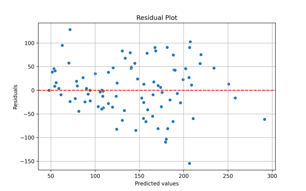
A key evaluation method is plotting residuals against a horizontal zero line.
This visualization helps assess whether linear regression assumptions are met. When residuals are evenly distributed around zero with no distinct patterns, the model likely satisfies these assumptions.
If residuals form non-random patterns (like curves or arcs), this suggests the relationships between variables aren’t linear—violating the linearity assumption.
A cone-shaped distribution, where the spread of residuals widens or narrows, indicates non-constant variance and violates the homoscedasticity assumption.
Residuals consistently appearing above or below the zero line suggest the presence of systematic bias in the model.
import matplotlib.pyplot as plt
import seaborn as sns
import numpy as np
# Calcolo residui
residuals = y_test - y_pred
# Plot residui vs valori predetti
plt.figure(figsize=(8, 5))
sns.scatterplot(x=y_pred, y=residuals)
plt.axhline(y=0, color='red', linestyle='--')
plt.xlabel('Predicted values')
plt.ylabel('Residuals')
plt.title('Residual Plot')
plt.grid(True)
plt.show()
```
import matplotlib.pyplot as plt
import seaborn as sns
import numpy as np
# Calcolo residui
residuals = y_test - y_pred
# Plot residui vs valori predetti
plt.figure(figsize=(8, 5))
sns.scatterplot(x=y_pred, y=residuals)
plt.axhline(y=0, color='red', linestyle='--')
plt.xlabel('Predicted values')
plt.ylabel('Residuals')
plt.title('Residual Plot')
plt.grid(True)
plt.show()
```
Based on this analysis, the model’s assumptions appear to be satisfied:
#### Residual Patterns
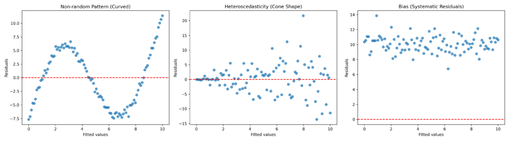
The graph reveals three main anomalous patterns in the residual curve:
Non-random Pattern (Curved): A distinct sinusoidal trend appears around the red line (zero value), indicating that the model fails to capture the non-linear relationship between variables.
Heteroscedasticity (Cone Shape): Residuals show increasing dispersion at higher fitted values, violating the assumption of constant variance (homoscedasticity).
Bias (Systematic Residuals): Predominantly positive residuals indicate that the model systematically underestimates values, possibly due to a missing intercept.
## How can we evaluate the quality of a linear regression model?
Several techniques exist for evaluating linear regression models. We’ll briefly cover these here, since we’ll dedicate an entire section later to Machine Learning model evaluation.
R² (coefficient of determination)→ Measures the proportion of target variance that the model explains.
MSE (Mean Squared Error)→ Mean of squared errors between predicted and observed values, which emphasizes large errors.
RMSE (Root Mean Squared Error)→ Square root of MSE, providing interpretable units matching the target variable.
MAE (Mean Absolute Error)→ Mean of absolute errors, providing a more robust measure less affected by outliers.
Residual Analysis→ Visual examination of errors to assess patterns, linearity, and variance consistency.
Residuals vs Predicted Values Plot→ Reveals potential heteroscedasticity or non-linearity issues.
Residual Distribution→ Tests for error normality using Shapiro-Wilk test, histograms, and QQ-plots.
Cross-validation (k-fold)→ Provides a realistic assessment of the model’s generalization ability.
Collinearity Test (VIF)→ Identifies problematic correlations among independent variables.
Adjusted Metrics (Adjusted R²)→ Accounts for model complexity by penalizing unnecessary variables in multiple regression.
## Linear Regression in Medicine
Linear regression is one of the most widely used statistical tests in medicine.
Through linear regression, researchers can evaluate relationships between clinical variables (like dose-response), identify predictors of outcomes (such as length of stay and blood pressure), develop prognostic and clinical decision support models, and analyze results from observational studies and clinical trials.
As illustrative examples, here are some studies that have employed this method.
Xia L, Zhang P, Niu JW, Ge W, Chen JT, Yang S, Su AX, Feng YZ, Wang F, Chen G, Chen GH. Relationships Between a Range of Inflammatory Biomarkers and Subjective Sleep Quality in Chronic Insomnia Patients: A Clinical Study. Nat Sci Sleep. 2021 Aug 12;13:1419-1428. doi: 10.2147/NSS.S310698
_Linear regression were used to explore the associations between the serum levels of inflammatory factors and the sleep quality._
Konstantopoulou G, Iliou T, Karaivazoglou K, Iconomou G, Assimakopoulos K, Alexopoulos P. Associations between (sub) clinical stress- and anxiety symptoms in mentally healthy individuals and in major depression: a cross-sectional clinical study. BMC Psychiatry. 2020 Sep 1;20(1):428. doi: 10.1186/s12888-020-02836-1
_Linear regression was used for studying the relationship between stress- and anxiety symptoms._
Nakajima K, Heilbrun LK, Hogan V, Smith D, Heath E, Raz A. Positive associations between galectin-3 and PSA levels in prostate cancer patients: a prospective clinical study-I. Oncotarget. 2016 Dec 13;7(50):82266-82272. doi: 10.18632/oncotarget.12619.
_To characterize the statistical relationship between relative Gal-3 and relative PSA, ordinary least squares (OLS) linear regression modeling was used._B1
## Additional Reading:
[StatQuest by Josh Starmer](https://youtu.be/nk2CQITm_eo)
[Wikipedia](https://en.wikipedia.org/wiki/Linear_regression)
[Scikit-learn](https://scikit-learn.org/stable/modules/generated/sklearn.linear_model.LinearRegression.html)
[Datacamp](https://www.datacamp.com/tutorial/simple-linear-regression)
## Conclusions
Linear regression is a fundamental statistical analysis tool that plays a central role in modern medicine, particularly for clinical predictions. Its strength lies in simplicity: it uses a linear equation to connect explanatory variables to outcomes of interest—such as diabetes progression or hospital stay duration—providing a clear, understandable model.
In medical settings, it enables physicians to measure the impact of clinical factors and identify modifiable risks. For accurate results, the model requires a linear relationship between variables, symmetrically distributed independent errors, and consistent error variance.
In today’s data-driven medicine, understanding linear regression fundamentals is crucial for interpreting quantitative evidence. This analytical tool effectively transforms data into clinical decisions, enabling doctors to make predictions, assess risks, and measure treatment effects.