---
title: Support Vector Machines
date: 2025-06-05T05:23:34Z
modified: 2026-07-22T05:29:46Z
permalink: "https://www.micheledpierri.com/machine-learning/support-vector-machines/"
type: page
status: publish
excerpt: ""
wpid: 1343
featured_image: "https://www.micheledpierri.com/wp-content/uploads/2026/07/ml_svm_.png"
featured_image_alt: A lone farmer travels along a dirt path dividing rows of purple lavender and golden sunflowers beneath a warm, hazy sky.
timestamp: 2026-07-22T05:29:46Z
tags: []
---
## Introduction
Support Vector Machines are supervised learning algorithms that primarily handle classification problems, though they can also perform regression tasks. They excel at finding boundaries between classes and are especially effective with high-dimensional data.
## Definition and Mathematical Foundations
### Definition
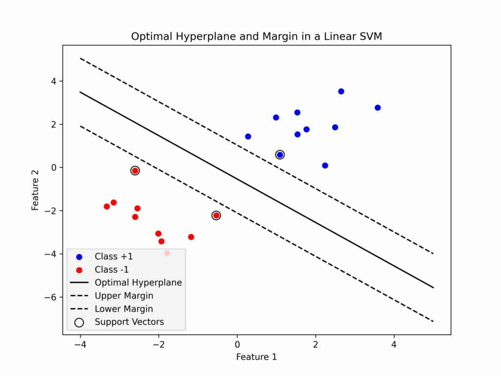
IIn binary classification, data is split into two classes. Support Vector Machines find the best boundary. This boundary is a line in 2D, a plane in 3D, or a hyperplane in higher dimensions.
This boundary is positioned to maximize the distance (called the margin) between points of different classes. The data points that lie exactly on the margin are known as “support vectors.”
### Mathematical Foundations
Given a set of points {(xi, yi)}, where x represents the feature vector and y represents the label, the hyperplane is defined as:

 is the weight vector, –  is the feature vector, –  is the bias.
The algorithm chooses a hyperplane that maximizes the margin between classes.
To identify the optimal margin, we need to solve:

When classes aren’t perfectly separable, we introduce slack variables to handle violations:
![\[ \min_{w, b, \xi} \frac{1}{2} ||w||^2 + C \sum_{i=1}^{N} \xi_i \]](https://www.micheledpierri.com/wp-content/ql-cache/quicklatex.com-90f726cda80b5a36b1d18aefd3a9a7cd_l3.svg "Rendered by QuickLaTeX.com")
where ![\[ y_i (w \cdot x_i + b) \geq 1 - \xi_i, \quad \forall i, \quad \xi_i \geq 0 \]](https://www.micheledpierri.com/wp-content/ql-cache/quicklatex.com-fefb435477718400b2c9f22d662331b0_l3.svg "Rendered by QuickLaTeX.com")
Here, C is a regularization parameter that we’ll explore further.
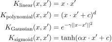
For data that cannot be separated linearly, kernel functions offer a solution by mapping the data into a higher-dimensional space where linear separation becomes possible.
Common kernel functions include:
### The C hyperparameter
The parameter C is a hyperparameter that balances between accurate classification of training data and effective generalization to new data.
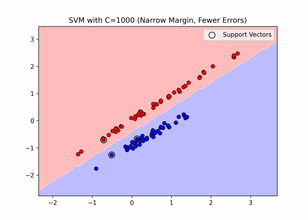
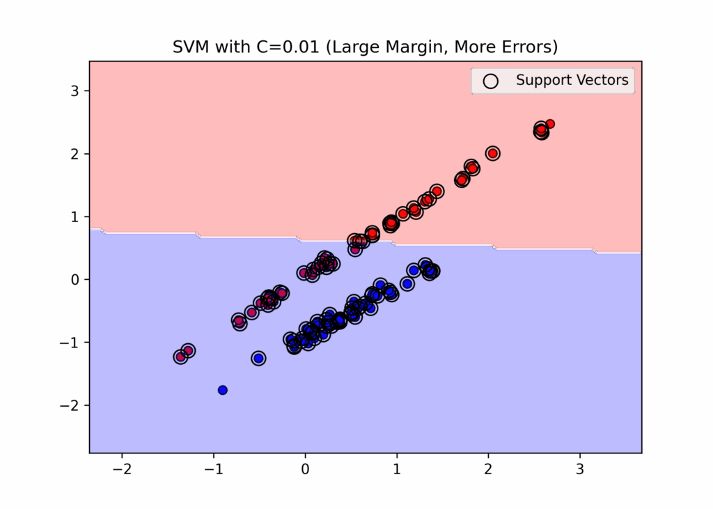
When C is set high, the model aims for perfect classification of all training points, but this increases the risk of overfitting. Conversely, a low C value allows some classification errors while widening the margin, which helps prevent overfitting.
When working with limited data or noisy datasets, it’s better to use a lower C value. However, when dealing with abundant, clearly separable data, a higher C value is more appropriate.
In the graphs, we deliberately set extreme values for C (both very small and very large) to demonstrate their effects on the margins. When C is small, the margins are wide, allowing for some misclassifications. When C is large, the margins become narrow and prevent any misclassifications.
## Medical Application
The medical literature contains numerous studies demonstrating Support Vector Machines’s successful applications and significant role in healthcare:
- cancer classification and diagnosis (Huang S, Cai N, Pacheco PP, Narrandes S, Wang Y, Xu W. Applications of Support Vector Machine (SVM) Learning in Cancer Genomics. Cancer Genomics Proteomics. 2018 Jan-Feb;15(1):41-51. doi: 10.21873/cgp.20063IF: 2.6 Q2 . PMID: 29275361; PMCID: PMC5822181.)
- classification and medication adherence (Son YJ, Kim HG, Kim EH, Choi S, Lee SK. Application of support vector machine for prediction of medication adherence in heart failure patients. Healthc Inform Res. 2010 Dec;16(4):253-9. doi: 10.4258/hir.2010.16.4.253. Epub 2010 Dec 31. PMID: 21818444; PMCID: PMC3092139.)
- use for diabetes and pre-diabetes diagnosis (Yu, W., Liu, T., Valdez, R. _et al._ Application of support vector machine modeling for prediction of common diseases: the case of diabetes and pre-diabetes. _BMC Med Inform Decis Mak_ **10**, 16 (2010). [https://doi.org/10.1186/1472-6947-10-16](https://doi.org/10.1186/1472-6947-10-16))
## Other Applications
Support Vector Machines have found extensive applications across numerous domains, demonstrating their versatility and effectiveness.
In computer vision, they are key for tasks like image classification, segmentation, and facial recognition.
In natural language processing, SVMs excel at text classification tasks, enabling the categorization of documents, filtering spam, and analyzing sentiment.
The algorithm processes audio for speech recognition and speaker identification.
In the financial sector, SVMs play a crucial role in fraud detection systems by analyzing transaction patterns to identify suspicious banking and credit card activities.
The industrial sector has also embraced SVMs for quality control and maintenance, implementing them in fault detection systems and continuous machine monitoring to predict and prevent equipment failures.
## When to Use Support Vector Machines
SVMs suit cases with limited data that has high dimensionality. They handle both linear and non-linear data effectively (thanks to kernel functions), and they perform well when you need a model that stays robust and resists outliers.
## Limitations of using Support Vector Machines
SVMs perform poorly with very large datasets (over 100,000 samples) and when processing irrelevant or low-quality features. With large datasets in particular, they demand substantial computational resources.
## Application in Python
We will employ Support Vector Machine (SVM) classification for breast tumor prediction by using a comprehensive dataset that is readily available within the scikit-learn library.
This dataset contains a rich collection of medical imaging data, with 30 distinct features carefully extracted from digital images of tumor masses. These features include various physical characteristics such as the radius of the mass, its perimeter measurements, detailed texture analysis, and several other relevant metrics that characterize the tumor’s properties. Each case in the dataset includes a binary classification indicating whether the tumor is benign or malignant, providing a clear target for our predictive modeling efforts.
After loading the dataset into a pandas DataFrame, we split the data into features (X) and target (y), then divided them into training (80%) and test (20%) sets. We normalized the features using StandardScaler and implemented an SVM algorithm with an “rbf” kernel—the most commonly used kernel type, particularly suitable for non-linear data. We set the hyperparameter C to 1.
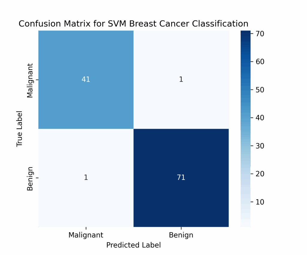
After training the model, we evaluated its performance using test data metrics and generated a confusion matrix with graphical visualization.
\# import necessary libraries since execution state was reset import numpy as np import matplotlib.pyplot as plt import seaborn as sns import pandas as pd from sklearn.datasets import load\_breast\_cancer from sklearn.model\_selection import train\_test\_split from sklearn.preprocessing import StandardScaler from sklearn.svm import SVC from sklearn.metrics import accuracy\_score, confusion\_matrix, classification\_report # Load the Breast Cancer dataset from scikit-learn cancer = load\_breast\_cancer() # Convert to a pandas DataFrame for better visualization df = pd.DataFrame(cancer.data, columns=cancer.feature\_names) df\[‘target’\] = cancer.target # Step 1: Data Preprocessing (Feature Scaling) X = df.drop(columns=\[‘target’\]) # Features (independent variables) y = df\[‘target’\] # Target variable (Malignant = 0, Benign = 1) # Split dataset into training (80%) and testing (20%) sets X\_train, X\_test, y\_train, y\_test = train\_test\_split(X, y, test\_size=0.2, random\_state=42, stratify=y) # Normalize the features using StandardScaler scaler = StandardScaler() X\_train\_scaled = scaler.fit\_transform(X\_train) X\_test\_scaled = scaler.transform(X\_test) # Step 2: Train the SVM Model svm\_model = SVC(kernel=”rbf”, C=1.0, gamma=”scale”) # Using an RBF Kernel for non-linearity svm\_model.fit(X\_train\_scaled, y\_train) # Step 3: Predictions and Model Evaluation y\_pred = svm\_model.predict(X\_test\_scaled) # Compute accuracy accuracy = accuracy\_score(y\_test, y\_pred) print(f”Model Accuracy: {accuracy:.2f}”) # Generate confusion matrix and classification report conf\_matrix = confusion\_matrix(y\_test, y\_pred) class\_report = classification\_report(y\_test, y\_pred, target\_names=\[“Malignant”, “Benign”\]) # Step 4: Visualizing Confusion Matrix plt.figure(figsize=(6,5)) sns.heatmap(conf\_matrix, annot=True, fmt=’d’, cmap=’Blues’, xticklabels=\[“Malignant”, “Benign”\], yticklabels=\[“Malignant”, “Benign”\]) plt.xlabel(“Predicted Label”) plt.ylabel(“True Label”) plt.title(“Confusion Matrix for SVM Breast Cancer Classification”) plt.show() # Display classification report print(“Classification Report:\\n”, class\_report) ```
# import necessary libraries since execution state was reset
import numpy as np
import matplotlib.pyplot as plt
import seaborn as sns
import pandas as pd
from sklearn.datasets import load_breast_cancer
from sklearn.model_selection import train_test_split
from sklearn.preprocessing import StandardScaler
from sklearn.svm import SVC
from sklearn.metrics import accuracy_score, confusion_matrix, classification_report
# Load the Breast Cancer dataset from scikit-learn
cancer = load_breast_cancer()
# Convert to a pandas DataFrame for better visualization
df = pd.DataFrame(cancer.data, columns=cancer.feature_names)
df['target'] = cancer.target
# Step 1: Data Preprocessing (Feature Scaling)
X = df.drop(columns=['target']) # Features (independent variables)
y = df['target'] # Target variable (Malignant = 0, Benign = 1)
# Split dataset into training (80%) and testing (20%) sets
X_train, X_test, y_train, y_test = train_test_split(X, y, test_size=0.2, random_state=42, stratify=y)
# Normalize the features using StandardScaler
scaler = StandardScaler()
X_train_scaled = scaler.fit_transform(X_train)
X_test_scaled = scaler.transform(X_test)
# Step 2: Train the SVM Model
svm_model = SVC(kernel="rbf", C=1.0, gamma="scale") # Using an RBF Kernel for non-linearity
svm_model.fit(X_train_scaled, y_train)
# Step 3: Predictions and Model Evaluation
y_pred = svm_model.predict(X_test_scaled)
# Compute accuracy
accuracy = accuracy_score(y_test, y_pred)
print(f"Model Accuracy: {accuracy:.2f}")
# Generate confusion matrix and classification report
conf_matrix = confusion_matrix(y_test, y_pred)
class_report = classification_report(y_test, y_pred, target_names=["Malignant", "Benign"])
# Step 4: Visualizing Confusion Matrix
plt.figure(figsize=(6,5))
sns.heatmap(conf_matrix, annot=True, fmt='d', cmap='Blues', xticklabels=["Malignant", "Benign"], yticklabels=["Malignant", "Benign"])
plt.xlabel("Predicted Label")
plt.ylabel("True Label")
plt.title("Confusion Matrix for SVM Breast Cancer Classification")
plt.show()
# Display classification report
print("Classification Report:\n", class_report)
```
The model achieves excellent performance, separating benign and malignant tumors with 98% accuracy. The visualization of the decision boundary and margins (created using PCA dimensionality reduction) shows that despite some overlap between classes, the model effectively differentiates between the two tumor types.
## Conclusion
Support Vector Machines demonstrate effectiveness in real-world scenarios where limited but feature-rich datasets exist, making them particularly valuable for specialized classification tasks. They handle high-dimensional data while maintaining good generalization, which makes them an excellent choice for many practical applications. However, their computational complexity limits their ability to process large-scale datasets. Despite their kernel capabilities, they may struggle with extremely complex non-linear relationships that require more sophisticated deep learning approaches.