---
title: Chi Square
date: 2024-11-05T08:38:27Z
modified: 2026-07-19T10:25:08Z
permalink: "https://www.micheledpierri.com/statistics/chi-square/"
type: page
status: publish
excerpt: ""
wpid: 795
featured_image: "https://www.micheledpierri.com/wp-content/uploads/2026/07/st_chi_square_.png"
featured_image_alt: An elderly scholar stands behind antique scales comparing “observed” and “expected” values in a softly lit historical apothecary.
timestamp: 2026-07-19T10:25:08Z
tags: []
---

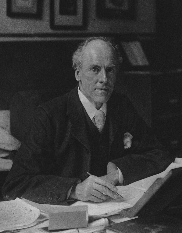
The chi-square test, developed by Karl Pearson—one of the founding fathers of statistics—in 1900, remains one of the most widely used statistical tools. Its popularity stems from its versatility and ease of application.
![Karl Pearson' photo](https://www.micheledpierri.com/wp-content/uploads/2024/11/Karl_Pearson.jpg)

## Data Characteristics

The chi-square test is suitable for categorical data—information grouped into discrete categories such as sex, color, or responses. These data are summarized in contingency tables, where each cell represents the frequency of a specific combination of characteristics.

Here’s an example of data suitable for a chi-square test: imagine comparing two treatments (A and B) with two possible outcomes (cured or not cured).

After our observation, we have:

- Treatment A 
    - 30 cured patients
    - 20 uncured patients
- Treatment B 
    - 50 cured patients
    - 25 uncured patients

We can structure this data in a contingency table:


| Cured | Not Cured | Total |  |
| --- | --- | --- | --- |
| Treatment A | 30 | 20 | 50 |
| Treatment B | 50 | 25 | 75 |
| Total | 80 | 45 | 125 |

These numbers represent the observed frequencies.

The chi-square test determines whether these observed frequencies differ significantly from the expected frequencies.

## Test Hypotheses

The null hypothesis (H₀) states that there are no significant differences between the observed distribution and the expected distribution.

The alternative hypothesis (H₁) proposes that the difference between the observed and expected distributions is not due to chance.

## Calculation of Expected Values

Of the 125 total patients, 50 underwent treatment A—40% (0.4) of the group. Additionally, 80 patients were cured, representing 64% (0.64) of the total. Therefore, we’d expect 25.6% of patients (0.4 × 0.64 = 0.256) to have undergone treatment A and been cured. In a group of 125, this translates to 32 patients (125 × 25.6%).

From this, we can derive a general formula to calculate the expected values for each combination:

![E_{ij} = \frac{(Total\ row_i) \times (Total\ column_j)}{Grand\ total}](https://www.micheledpierri.com/wp-content/ql-cache/quicklatex.com-c0ebc3211750aee6f97b11d853ec6bb2_l3.svg "Rendered by QuickLaTeX.com")

Using this formula, we can calculate the expected value for each observed value:


| Cured (O) | Not Cured (O) | Cured (E) | Not Cured (E) | Total |  |
| --- | --- | --- | --- | --- | --- |
| Treatment A | 30 | 20 | 32 | 18 | 50 |
| Treatment B | 50 | 25 | 48 | 27 | 75 |

O = Observed, E = Expected## Calculation of χ²

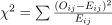
The chi-square (χ²) statistic is calculated by summing the squares of the differences between observed and expected values for each cell, divided by the expected value for that cell:
![\chi^2 = \sum \frac{(O_{ij} - E_{ij})^2}{E_{ij}}](https://www.micheledpierri.com/wp-content/ql-cache/quicklatex.com-6cc84eaefa2306a886f6c28fa54649c8_l3.svg "Rendered by QuickLaTeX.com")

In this formula, O represents the observed frequency, and E represents the expected frequency.

A higher χ² value indicates a greater discrepancy between observed and expected values, suggesting that the difference is less likely to be due to chance.

## Degrees of Freedom and P-value: The χ² Distribution

To calculate the p-value of the chi-square test, we need to determine the degrees of freedom. For a table with c columns and r rows, the formula is:

(r-1) × (c-1)

Using these parameters, we can derive the p-value. If it’s less than 0.05, we reject the null hypothesis and accept the alternative hypothesis—indicating that the difference from the expected values is not due to chance.

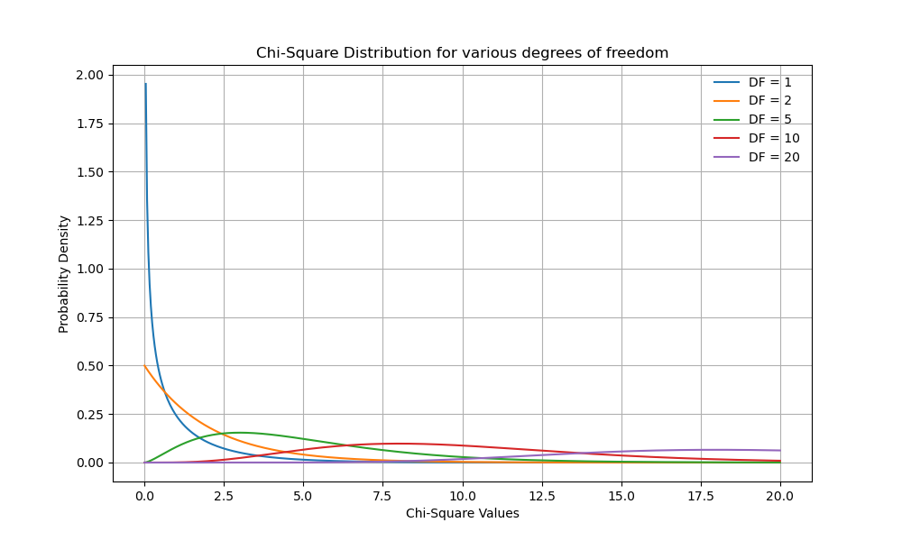
The p-value is determined based on the chi-square distribution. The tail of this distribution—the rightmost part of the graph—represents the rejection area for the null hypothesis. The chi-square distribution is positive, with a curve featuring a tail that extends infinitely to the right. Interestingly, the curve’s asymmetry depends on the degrees of freedom: as these increase, the curve becomes more symmetrical, gradually resembling a normal distribution curve.
![Chi square distribution for various degrees of freedom](https://www.micheledpierri.com/wp-content/uploads/2024/11/chi_square1.png)

## Limitations of χ²

The chi-square test, while widely used, has several important limitations:

- Sample Size Sensitivity: Large samples can lead to statistically significant results even for minor differences between observed and expected values, potentially overestimating the practical significance.
- Low Expected Frequencies: The test’s reliability decreases when expected frequencies in some cells are low (typically less than 5), which can lead to inaccurate results.
- Association Only: While the test can establish the existence of an association, it doesn’t provide information about the direction or strength of that association.
- Assumes Independence: The test assumes that each observation is independent, which may not always be the case in real-world scenarios.

To address these limitations, researchers can employ alternative or complementary methods:

- Fisher’s Exact Test: Suitable for small sample sizes or when expected frequencies are low.
- Cramer’s V: Assesses the strength of association between categorical variables.
- Log-linear Analysis: Allows for more complex analyses of multi-way contingency tables.
- Bootstrapping Techniques: Can provide more robust estimates for small samples.

## χ² in Python

Let’s explore a practical application by creating a hypothetical dataset of patients undergoing various treatments and their outcomes.

import numpy as np
import pandas as pd
import matplotlib.pyplot as plt
import seaborn as sns
from scipy.stats import chi2_contingency

# Step 1: Create a fictional dataset
# Columns: Treatment Type, Recovery Outcome (Counts)
data = {'Treatment': ['Treatment A', 'Treatment A', 'Treatment B', 'Treatment B'],
        'Outcome': ['Recovered', 'Not Recovered', 'Recovered', 'Not Recovered'],
        'Count': [50, 30, 45, 55]}
df = pd.DataFrame(data)

# Step 2: Pivot the dataset to form a contingency table
contingency_table = df.pivot(index='Treatment', columns='Outcome', values='Count')

# Step 3: Perform the chi-square test
chi2, p_value, dof, expected = chi2_contingency(contingency_table)

# Convert expected frequencies to DataFrame for easier plotting
expected_df = pd.DataFrame(expected, index=contingency_table.index, columns=contingency_table.columns)

# Step 4: Display results
print("Chi-square Statistic:", chi2)
print("P-value:", p_value)
print("Degrees of Freedom:", dof)
print("Expected Frequencies:\n", expected_df)

# Step 5: Plot observed and expected frequencies
plt.figure(figsize=(12, 5))

# Observed Frequencies
plt.subplot(1, 2, 1)
sns.barplot(x='Outcome', y='Count', hue='Treatment', data=df)
plt.title("Observed Frequencies")
plt.ylabel("Number of Patients")

# Expected Frequencies
plt.subplot(1, 2, 2)
expected_long = expected_df.reset_index().melt(id_vars='Treatment', value_name='Expected Count')
sns.barplot(x='Outcome', y='Expected Count', hue='Treatment', data=expected_long)
plt.title("Expected Frequencies")
plt.ylabel("Expected Number of Patients")

plt.tight_layout()
plt.show()
```
<span class="line"><span style="color: #FF79C6">import</span><span style="color: #F8F8F2"> numpy </span><span style="color: #FF79C6">as</span><span style="color: #F8F8F2"> np</span></span>
<span class="line"><span style="color: #FF79C6">import</span><span style="color: #F8F8F2"> pandas </span><span style="color: #FF79C6">as</span><span style="color: #F8F8F2"> pd</span></span>
<span class="line"><span style="color: #FF79C6">import</span><span style="color: #F8F8F2"> matplotlib.pyplot </span><span style="color: #FF79C6">as</span><span style="color: #F8F8F2"> plt</span></span>
<span class="line"><span style="color: #FF79C6">import</span><span style="color: #F8F8F2"> seaborn </span><span style="color: #FF79C6">as</span><span style="color: #F8F8F2"> sns</span></span>
<span class="line"><span style="color: #FF79C6">from</span><span style="color: #F8F8F2"> scipy.stats </span><span style="color: #FF79C6">import</span><span style="color: #F8F8F2"> chi2_contingency</span></span>
<span class="line"></span>
<span class="line"><span style="color: #6272A4"># Step 1: Create a fictional dataset</span></span>
<span class="line"><span style="color: #6272A4"># Columns: Treatment Type, Recovery Outcome (Counts)</span></span>
<span class="line"><span style="color: #F8F8F2">data </span><span style="color: #FF79C6">=</span><span style="color: #F8F8F2"> {</span><span style="color: #E9F284">'</span><span style="color: #F1FA8C">Treatment</span><span style="color: #E9F284">'</span><span style="color: #F8F8F2">: [</span><span style="color: #E9F284">'</span><span style="color: #F1FA8C">Treatment A</span><span style="color: #E9F284">'</span><span style="color: #F8F8F2">, </span><span style="color: #E9F284">'</span><span style="color: #F1FA8C">Treatment A</span><span style="color: #E9F284">'</span><span style="color: #F8F8F2">, </span><span style="color: #E9F284">'</span><span style="color: #F1FA8C">Treatment B</span><span style="color: #E9F284">'</span><span style="color: #F8F8F2">, </span><span style="color: #E9F284">'</span><span style="color: #F1FA8C">Treatment B</span><span style="color: #E9F284">'</span><span style="color: #F8F8F2">],</span></span>
<span class="line"><span style="color: #F8F8F2">        </span><span style="color: #E9F284">'</span><span style="color: #F1FA8C">Outcome</span><span style="color: #E9F284">'</span><span style="color: #F8F8F2">: [</span><span style="color: #E9F284">'</span><span style="color: #F1FA8C">Recovered</span><span style="color: #E9F284">'</span><span style="color: #F8F8F2">, </span><span style="color: #E9F284">'</span><span style="color: #F1FA8C">Not Recovered</span><span style="color: #E9F284">'</span><span style="color: #F8F8F2">, </span><span style="color: #E9F284">'</span><span style="color: #F1FA8C">Recovered</span><span style="color: #E9F284">'</span><span style="color: #F8F8F2">, </span><span style="color: #E9F284">'</span><span style="color: #F1FA8C">Not Recovered</span><span style="color: #E9F284">'</span><span style="color: #F8F8F2">],</span></span>
<span class="line"><span style="color: #F8F8F2">        </span><span style="color: #E9F284">'</span><span style="color: #F1FA8C">Count</span><span style="color: #E9F284">'</span><span style="color: #F8F8F2">: [</span><span style="color: #BD93F9">50</span><span style="color: #F8F8F2">, </span><span style="color: #BD93F9">30</span><span style="color: #F8F8F2">, </span><span style="color: #BD93F9">45</span><span style="color: #F8F8F2">, </span><span style="color: #BD93F9">55</span><span style="color: #F8F8F2">]}</span></span>
<span class="line"><span style="color: #F8F8F2">df </span><span style="color: #FF79C6">=</span><span style="color: #F8F8F2"> pd.DataFrame(data)</span></span>
<span class="line"></span>
<span class="line"><span style="color: #6272A4"># Step 2: Pivot the dataset to form a contingency table</span></span>
<span class="line"><span style="color: #F8F8F2">contingency_table </span><span style="color: #FF79C6">=</span><span style="color: #F8F8F2"> df.pivot(</span><span style="color: #FFB86C; font-style: italic">index</span><span style="color: #FF79C6">=</span><span style="color: #E9F284">'</span><span style="color: #F1FA8C">Treatment</span><span style="color: #E9F284">'</span><span style="color: #F8F8F2">, </span><span style="color: #FFB86C; font-style: italic">columns</span><span style="color: #FF79C6">=</span><span style="color: #E9F284">'</span><span style="color: #F1FA8C">Outcome</span><span style="color: #E9F284">'</span><span style="color: #F8F8F2">, </span><span style="color: #FFB86C; font-style: italic">values</span><span style="color: #FF79C6">=</span><span style="color: #E9F284">'</span><span style="color: #F1FA8C">Count</span><span style="color: #E9F284">'</span><span style="color: #F8F8F2">)</span></span>
<span class="line"></span>
<span class="line"><span style="color: #6272A4"># Step 3: Perform the chi-square test</span></span>
<span class="line"><span style="color: #F8F8F2">chi2, p_value, dof, expected </span><span style="color: #FF79C6">=</span><span style="color: #F8F8F2"> chi2_contingency(contingency_table)</span></span>
<span class="line"></span>
<span class="line"><span style="color: #6272A4"># Convert expected frequencies to DataFrame for easier plotting</span></span>
<span class="line"><span style="color: #F8F8F2">expected_df </span><span style="color: #FF79C6">=</span><span style="color: #F8F8F2"> pd.DataFrame(expected, </span><span style="color: #FFB86C; font-style: italic">index</span><span style="color: #FF79C6">=</span><span style="color: #F8F8F2">contingency_table.index, </span><span style="color: #FFB86C; font-style: italic">columns</span><span style="color: #FF79C6">=</span><span style="color: #F8F8F2">contingency_table.columns)</span></span>
<span class="line"></span>
<span class="line"><span style="color: #6272A4"># Step 4: Display results</span></span>
<span class="line"><span style="color: #8BE9FD">print</span><span style="color: #F8F8F2">(</span><span style="color: #E9F284">"</span><span style="color: #F1FA8C">Chi-square Statistic:</span><span style="color: #E9F284">"</span><span style="color: #F8F8F2">, chi2)</span></span>
<span class="line"><span style="color: #8BE9FD">print</span><span style="color: #F8F8F2">(</span><span style="color: #E9F284">"</span><span style="color: #F1FA8C">P-value:</span><span style="color: #E9F284">"</span><span style="color: #F8F8F2">, p_value)</span></span>
<span class="line"><span style="color: #8BE9FD">print</span><span style="color: #F8F8F2">(</span><span style="color: #E9F284">"</span><span style="color: #F1FA8C">Degrees of Freedom:</span><span style="color: #E9F284">"</span><span style="color: #F8F8F2">, dof)</span></span>
<span class="line"><span style="color: #8BE9FD">print</span><span style="color: #F8F8F2">(</span><span style="color: #E9F284">"</span><span style="color: #F1FA8C">Expected Frequencies:</span><span style="color: #FF79C6">\n</span><span style="color: #E9F284">"</span><span style="color: #F8F8F2">, expected_df)</span></span>
<span class="line"></span>
<span class="line"><span style="color: #6272A4"># Step 5: Plot observed and expected frequencies</span></span>
<span class="line"><span style="color: #F8F8F2">plt.figure(</span><span style="color: #FFB86C; font-style: italic">figsize</span><span style="color: #FF79C6">=</span><span style="color: #F8F8F2">(</span><span style="color: #BD93F9">12</span><span style="color: #F8F8F2">, </span><span style="color: #BD93F9">5</span><span style="color: #F8F8F2">))</span></span>
<span class="line"></span>
<span class="line"><span style="color: #6272A4"># Observed Frequencies</span></span>
<span class="line"><span style="color: #F8F8F2">plt.subplot(</span><span style="color: #BD93F9">1</span><span style="color: #F8F8F2">, </span><span style="color: #BD93F9">2</span><span style="color: #F8F8F2">, </span><span style="color: #BD93F9">1</span><span style="color: #F8F8F2">)</span></span>
<span class="line"><span style="color: #F8F8F2">sns.barplot(</span><span style="color: #FFB86C; font-style: italic">x</span><span style="color: #FF79C6">=</span><span style="color: #E9F284">'</span><span style="color: #F1FA8C">Outcome</span><span style="color: #E9F284">'</span><span style="color: #F8F8F2">, </span><span style="color: #FFB86C; font-style: italic">y</span><span style="color: #FF79C6">=</span><span style="color: #E9F284">'</span><span style="color: #F1FA8C">Count</span><span style="color: #E9F284">'</span><span style="color: #F8F8F2">, </span><span style="color: #FFB86C; font-style: italic">hue</span><span style="color: #FF79C6">=</span><span style="color: #E9F284">'</span><span style="color: #F1FA8C">Treatment</span><span style="color: #E9F284">'</span><span style="color: #F8F8F2">, </span><span style="color: #FFB86C; font-style: italic">data</span><span style="color: #FF79C6">=</span><span style="color: #F8F8F2">df)</span></span>
<span class="line"><span style="color: #F8F8F2">plt.title(</span><span style="color: #E9F284">"</span><span style="color: #F1FA8C">Observed Frequencies</span><span style="color: #E9F284">"</span><span style="color: #F8F8F2">)</span></span>
<span class="line"><span style="color: #F8F8F2">plt.ylabel(</span><span style="color: #E9F284">"</span><span style="color: #F1FA8C">Number of Patients</span><span style="color: #E9F284">"</span><span style="color: #F8F8F2">)</span></span>
<span class="line"></span>
<span class="line"><span style="color: #6272A4"># Expected Frequencies</span></span>
<span class="line"><span style="color: #F8F8F2">plt.subplot(</span><span style="color: #BD93F9">1</span><span style="color: #F8F8F2">, </span><span style="color: #BD93F9">2</span><span style="color: #F8F8F2">, </span><span style="color: #BD93F9">2</span><span style="color: #F8F8F2">)</span></span>
<span class="line"><span style="color: #F8F8F2">expected_long </span><span style="color: #FF79C6">=</span><span style="color: #F8F8F2"> expected_df.reset_index().melt(</span><span style="color: #FFB86C; font-style: italic">id_vars</span><span style="color: #FF79C6">=</span><span style="color: #E9F284">'</span><span style="color: #F1FA8C">Treatment</span><span style="color: #E9F284">'</span><span style="color: #F8F8F2">, </span><span style="color: #FFB86C; font-style: italic">value_name</span><span style="color: #FF79C6">=</span><span style="color: #E9F284">'</span><span style="color: #F1FA8C">Expected Count</span><span style="color: #E9F284">'</span><span style="color: #F8F8F2">)</span></span>
<span class="line"><span style="color: #F8F8F2">sns.barplot(</span><span style="color: #FFB86C; font-style: italic">x</span><span style="color: #FF79C6">=</span><span style="color: #E9F284">'</span><span style="color: #F1FA8C">Outcome</span><span style="color: #E9F284">'</span><span style="color: #F8F8F2">, </span><span style="color: #FFB86C; font-style: italic">y</span><span style="color: #FF79C6">=</span><span style="color: #E9F284">'</span><span style="color: #F1FA8C">Expected Count</span><span style="color: #E9F284">'</span><span style="color: #F8F8F2">, </span><span style="color: #FFB86C; font-style: italic">hue</span><span style="color: #FF79C6">=</span><span style="color: #E9F284">'</span><span style="color: #F1FA8C">Treatment</span><span style="color: #E9F284">'</span><span style="color: #F8F8F2">, </span><span style="color: #FFB86C; font-style: italic">data</span><span style="color: #FF79C6">=</span><span style="color: #F8F8F2">expected_long)</span></span>
<span class="line"><span style="color: #F8F8F2">plt.title(</span><span style="color: #E9F284">"</span><span style="color: #F1FA8C">Expected Frequencies</span><span style="color: #E9F284">"</span><span style="color: #F8F8F2">)</span></span>
<span class="line"><span style="color: #F8F8F2">plt.ylabel(</span><span style="color: #E9F284">"</span><span style="color: #F1FA8C">Expected Number of Patients</span><span style="color: #E9F284">"</span><span style="color: #F8F8F2">)</span></span>
<span class="line"></span>
<span class="line"><span style="color: #F8F8F2">plt.tight_layout()</span></span>
<span class="line"><span style="color: #F8F8F2">plt.show()</span></span>
<span class="line"></span>
```

![Bar plot of observed vs espected frequencies](https://www.micheledpierri.com/wp-content/uploads/2024/11/chi_square2-1024x427.png)

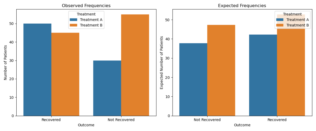
The test results show a chi-square statistic of 4.78 with 1 degree of freedom, yielding a p-value of 0.028. This outcome suggests a statistically significant difference between the observed and expected values.

Chi-square Statistic: 4.78170278637771
P-value: 0.028763665017943585
Degrees of Freedom: 1
Expected Frequencies:
 Outcome      Not Recovered  Recovered
Treatment                            
Treatment A      37.777778  42.222222
Treatment B      47.222222  52.777778```
<span class="line"><span style="color: #50FA7B">Chi-square</span><span style="color: #F8F8F2"> </span><span style="color: #F1FA8C">Statistic:</span><span style="color: #F8F8F2"> </span><span style="color: #BD93F9">4.78170278637771</span></span>
<span class="line"><span style="color: #50FA7B">P-value:</span><span style="color: #F8F8F2"> </span><span style="color: #BD93F9">0.028763665017943585</span></span>
<span class="line"><span style="color: #50FA7B">Degrees</span><span style="color: #F8F8F2"> </span><span style="color: #F1FA8C">of</span><span style="color: #F8F8F2"> </span><span style="color: #F1FA8C">Freedom:</span><span style="color: #F8F8F2"> </span><span style="color: #BD93F9">1</span></span>
<span class="line"><span style="color: #50FA7B">Expected</span><span style="color: #F8F8F2"> </span><span style="color: #F1FA8C">Frequencies:</span></span>
<span class="line"><span style="color: #F8F8F2"> </span><span style="color: #50FA7B">Outcome</span><span style="color: #F8F8F2">      </span><span style="color: #F1FA8C">Not</span><span style="color: #F8F8F2"> </span><span style="color: #F1FA8C">Recovered</span><span style="color: #F8F8F2">  </span><span style="color: #F1FA8C">Recovered</span></span>
<span class="line"><span style="color: #50FA7B">Treatment</span><span style="color: #F8F8F2">                            </span></span>
<span class="line"><span style="color: #50FA7B">Treatment</span><span style="color: #F8F8F2"> </span><span style="color: #F1FA8C">A</span><span style="color: #F8F8F2">      </span><span style="color: #BD93F9">37.777778</span><span style="color: #F8F8F2">  </span><span style="color: #BD93F9">42.222222</span></span>
<span class="line"><span style="color: #50FA7B">Treatment</span><span style="color: #F8F8F2"> </span><span style="color: #F1FA8C">B</span><span style="color: #F8F8F2">      </span><span style="color: #BD93F9">47.222222</span><span style="color: #F8F8F2">  </span><span style="color: #BD93F9">52.777778</span></span>
```