---
title: Monte Carlo Simulation
date: 2025-02-02T10:25:02Z
modified: 2026-07-20T19:28:48Z
permalink: "https://www.micheledpierri.com/statistics/monte-carlo-simulation/"
type: page
status: publish
excerpt: ""
wpid: 984
featured_image: "https://www.micheledpierri.com/wp-content/uploads/2026/07/st_monte_carlo_.png"
featured_image_alt: A Renaissance scholar studies dice on an ornate table in a medical study, framed by stone arches overlooking a sunlit historic city.
timestamp: 2026-07-20T19:28:48Z
tags: []
---

## Overview and Methodology

Monte Carlo simulation is a statistical tool used for problems with uncertain solutions, particularly those involving multiple variables with unknown values.

It runs multiple simulations of the problem, generating random values for the relevant variables each time.

The method takes its name from Monte Carlo, a city famous for its gambling and games of chance, reflecting how the simulation uses randomly generated variables.

At its core, Monte Carlo simulation relies on variables that have unknown values but follow known distributions. The method generates random values for these variables thousands or millions of times. This process yields important statistical metrics—like means and distributions—which form the basis for the final results.

Beyond the variables themselves, the simulation requires a model that connects these variables to the outcome.

## Applications in Medicine

- Risk Prediction: Monte Carlo methods help predict event risks in oncology and other medical fields by analyzing multiple variables.
- Treatment Outcome Assessment: The simulation predicts treatment outcomes effectively, even when working with uncertain clinical data.
- Healthcare Policy Evaluation: Monte Carlo simulations assess the potential outcomes of mass screening programs and healthcare policy initiatives.
- Resource Management: The method helps evaluate and predict patient loads across hospitals, departments, and individual wards.

## Operating Procedures

To perform a Monte Carlo evaluation, you need to:

- Analyze the variables involved in the phenomenon or process under study. In medicine, these typically include age, sex, weight, and—depending on the research focus—clinical data and therapeutic indicators.
- Determine the statistical distribution for each chosen variable. These may be normal or Gaussian for continuous variables (like age or blood pressure), binomial for two-value variables (sick/healthy, pathological/normal, alive/dead), or Poisson for repeated binomial variables.
- Establish the model that connects variables to outcomes. This can be done empirically (through statistical analysis of available data), theoretically (such as using pharmacokinetic laws for drug studies), or through a mixed approach combining both empirical and theoretical data.

With this information in hand, we can implement the Monte Carlo simulation. Based on the variables’ distribution characteristics and our model, the simulation runs thousands of iterations using random data values and tracks their effect on outcomes. The analysis of these numerous iterations produces a results distribution that informs decision-making.

## Problems and Limitations

To perform a Monte Carlo simulation, three key elements are essential: identified variables, known distributions for those variables, and a model that connects them to the desired outcome or process.

A significant challenge arises when variable distributions are unclear, particularly with limited available data.

Model development presents another hurdle—a model that’s too simplified may not reflect reality, while an overly complex one becomes difficult to implement and validate.

In medical applications, particularly for risk assessment, statistical regression typically forms the foundation of the model.

The process involves incorporating observational or experimental clinical study data into a regression model—whether linear, logistic, or Cox for survival data—to link variables to outcomes. These models provide valuable accuracy metrics (r-squared, AUC, Log-rank, etc.) before their integration into the Monte Carlo simulation.

## Practical Benefits

Monte Carlo simulation extends beyond traditional statistical models derived from observational or experimental clinical studies. While conventional linear or logistic regression models estimate outcomes based on mean values from initial data, Monte Carlo offers more.

The simulation generates random values across the full range of input data, revealing how outcomes change with varying conditions. This approach provides a comprehensive view of possible outcomes based on mean values and across the entire distribution of independent variables. As a result, we can generate detailed risk distribution curves.

This capability allows us to explore multiple scenarios, such as comparing outcomes for patients with high, medium, or low input values, and identifying critical risk thresholds.enabling users to analyze real data with ease while providing flexibility, computational efficiency, and seamless integration with Python’s scientific ecosystem.

## Monte Carlo Simulation in Python

Python offers several standard libraries for implementing Monte Carlo simulations, including NumPy, SciPy, Pandas, and Matplotlib.

The NumPy library’s powerful random number generation capabilities provide everything needed to simulate events with specific distributions in defined ranges.

For example, to simulate an age distribution from 20 to 80 years with a uniform distribution, you can use this simple code:

 ages = np.random.uniform(20, 80, num\_patients) ```
<span class="line"><span style="color: #F8F8F2"> ages </span><span style="color: #FF79C6">=</span><span style="color: #F8F8F2"> np.random.uniform(</span><span style="color: #BD93F9">20</span><span style="color: #F8F8F2">, </span><span style="color: #BD93F9">80</span><span style="color: #F8F8F2">, num_patients)</span></span>
<span class="line"></span>
```

Or to simulate a binary variable, such as whether a treatment is applied:

treatment = np.random.choice(\[0, 1\], size=num\_patients) ```
<span class="line"><span style="color: #F8F8F2">treatment </span><span style="color: #FF79C6">=</span><span style="color: #F8F8F2"> np.random.choice([</span><span style="color: #BD93F9">0</span><span style="color: #F8F8F2">, </span><span style="color: #BD93F9">1</span><span style="color: #F8F8F2">], </span><span style="color: #FFB86C; font-style: italic">size</span><span style="color: #FF79C6">=</span><span style="color: #F8F8F2">num_patients)</span></span>
<span class="line"></span>
```

For more complex Monte Carlo simulations, specialized libraries are available: PyMC3 for Bayesian statistics and TensorFlow Probability for stochastic simulations.

## Example 1: Survival Simulation with Monte Carlo Simulation

Consider a scenario with a patient’s annual survival rate of 85% (p=0.85).

The model has two key parameters: the total number of patients (n) and the annual survival probability (p).

Events follow a binomial distribution based on n and p:

![X \sim \text{Binomial}(n,p)](https://www.micheledpierri.com/wp-content/ql-cache/quicklatex.com-dc2ddf72173f294320bec42bae0a61c8_l3.svg "Rendered by QuickLaTeX.com")

For cumulative survival, patients who survive at year’s end become the exposed population for the following year:

![n_{t+1} = \text{Binomial}(n_t, p)](https://www.micheledpierri.com/wp-content/ql-cache/quicklatex.com-b29285a136175a0b544ca2ac5380c6e6_l3.svg "Rendered by QuickLaTeX.com")

This model is admittedly simplistic. It assumes both patient independence and a constant annual survival rate across all patients and years—assumptions that don’t reflect reality.

However, it serves well to demonstrate Monte Carlo simulation.

Below is the commented Python code:

Required Python Libraries:

import numpy as np import matplotlib.pyplot as plt import pandas as pd ```
<span class="line"></span>
<span class="line"><span style="color: #FF79C6">import</span><span style="color: #F8F8F2"> numpy </span><span style="color: #FF79C6">as</span><span style="color: #F8F8F2"> np</span></span>
<span class="line"><span style="color: #FF79C6">import</span><span style="color: #F8F8F2"> matplotlib.pyplot </span><span style="color: #FF79C6">as</span><span style="color: #F8F8F2"> plt</span></span>
<span class="line"><span style="color: #FF79C6">import</span><span style="color: #F8F8F2"> pandas </span><span style="color: #FF79C6">as</span><span style="color: #F8F8F2"> pd</span></span>
<span class="line"></span>
```

Step 1: define the simulation parameters

np.random.seed(42) # Setting seed for reproducibility num\_patients = 1000 # Number of patients in the study num\_simulations = 1000 # Number of Monte Carlo iterations survival\_probability\_yearly = 0.85 # Probability of survival each year num\_years = 5 # Total number of years to simulate ```
<span class="line"><span style="color: #F8F8F2">np.random.seed(</span><span style="color: #BD93F9">42</span><span style="color: #F8F8F2">)  </span><span style="color: #6272A4"># Setting seed for reproducibility</span></span>
<span class="line"><span style="color: #F8F8F2">num_patients </span><span style="color: #FF79C6">=</span><span style="color: #F8F8F2"> </span><span style="color: #BD93F9">1000</span><span style="color: #F8F8F2">  </span><span style="color: #6272A4"># Number of patients in the study</span></span>
<span class="line"><span style="color: #F8F8F2">num_simulations </span><span style="color: #FF79C6">=</span><span style="color: #F8F8F2"> </span><span style="color: #BD93F9">1000</span><span style="color: #F8F8F2">  </span><span style="color: #6272A4"># Number of Monte Carlo iterations</span></span>
<span class="line"><span style="color: #F8F8F2">survival_probability_yearly </span><span style="color: #FF79C6">=</span><span style="color: #F8F8F2"> </span><span style="color: #BD93F9">0.85</span><span style="color: #F8F8F2">  </span><span style="color: #6272A4"># Probability of survival each year</span></span>
<span class="line"><span style="color: #F8F8F2">num_years </span><span style="color: #FF79C6">=</span><span style="color: #F8F8F2"> </span><span style="color: #BD93F9">5</span><span style="color: #F8F8F2">  </span><span style="color: #6272A4"># Total number of years to simulate</span></span>
<span class="line"></span>
```

Step 2: create an array to store results of each simulation and runs the simulation

survival\_data = np.zeros((num\_simulations, num\_years)) for sim in range(num\_simulations): # Start with all patients alive survivors = num\_patients for year in range(num\_years): # Simulate survival for the current year based on survivors from the previous year survivors = np.random.binomial(survivors, survival\_probability\_yearly) survival\_data\[sim, year\] = survivors / num\_patients \* 100 # Store survival as percentag ```
<span class="line"><span style="color: #F8F8F2">survival_data </span><span style="color: #FF79C6">=</span><span style="color: #F8F8F2"> np.zeros((num_simulations, num_years))</span></span>
<span class="line"></span>
<span class="line"><span style="color: #FF79C6">for</span><span style="color: #F8F8F2"> sim </span><span style="color: #FF79C6">in</span><span style="color: #F8F8F2"> </span><span style="color: #8BE9FD">range</span><span style="color: #F8F8F2">(num_simulations):</span></span>
<span class="line"><span style="color: #F8F8F2">    </span><span style="color: #6272A4"># Start with all patients alive</span></span>
<span class="line"><span style="color: #F8F8F2">    survivors </span><span style="color: #FF79C6">=</span><span style="color: #F8F8F2"> num_patients</span></span>
<span class="line"><span style="color: #F8F8F2">    </span><span style="color: #FF79C6">for</span><span style="color: #F8F8F2"> year </span><span style="color: #FF79C6">in</span><span style="color: #F8F8F2"> </span><span style="color: #8BE9FD">range</span><span style="color: #F8F8F2">(num_years):</span></span>
<span class="line"><span style="color: #F8F8F2">        </span><span style="color: #6272A4"># Simulate survival for the current year based on survivors from the previous year</span></span>
<span class="line"><span style="color: #F8F8F2">        survivors </span><span style="color: #FF79C6">=</span><span style="color: #F8F8F2"> np.random.binomial(survivors, survival_probability_yearly)</span></span>
<span class="line"><span style="color: #F8F8F2">        survival_data[sim, year] </span><span style="color: #FF79C6">=</span><span style="color: #F8F8F2"> survivors </span><span style="color: #FF79C6">/</span><span style="color: #F8F8F2"> num_patients </span><span style="color: #FF79C6">*</span><span style="color: #F8F8F2"> </span><span style="color: #BD93F9">100</span><span style="color: #F8F8F2">  </span><span style="color: #6272A4"># Store survival as percentag</span></span>
<span class="line"></span>
```

Step 3: calculate metrics

mean\_survival = survival\_data.mean(axis=0) std\_survival = survival\_data.std(axis=0) ```
<span class="line"><span style="color: #F8F8F2">mean_survival </span><span style="color: #FF79C6">=</span><span style="color: #F8F8F2"> survival_data.mean(</span><span style="color: #FFB86C; font-style: italic">axis</span><span style="color: #FF79C6">=</span><span style="color: #BD93F9">0</span><span style="color: #F8F8F2">)</span></span>
<span class="line"><span style="color: #F8F8F2">std_survival </span><span style="color: #FF79C6">=</span><span style="color: #F8F8F2"> survival_data.std(</span><span style="color: #FFB86C; font-style: italic">axis</span><span style="color: #FF79C6">=</span><span style="color: #BD93F9">0</span><span style="color: #F8F8F2">)</span></span>
<span class="line"></span>
```

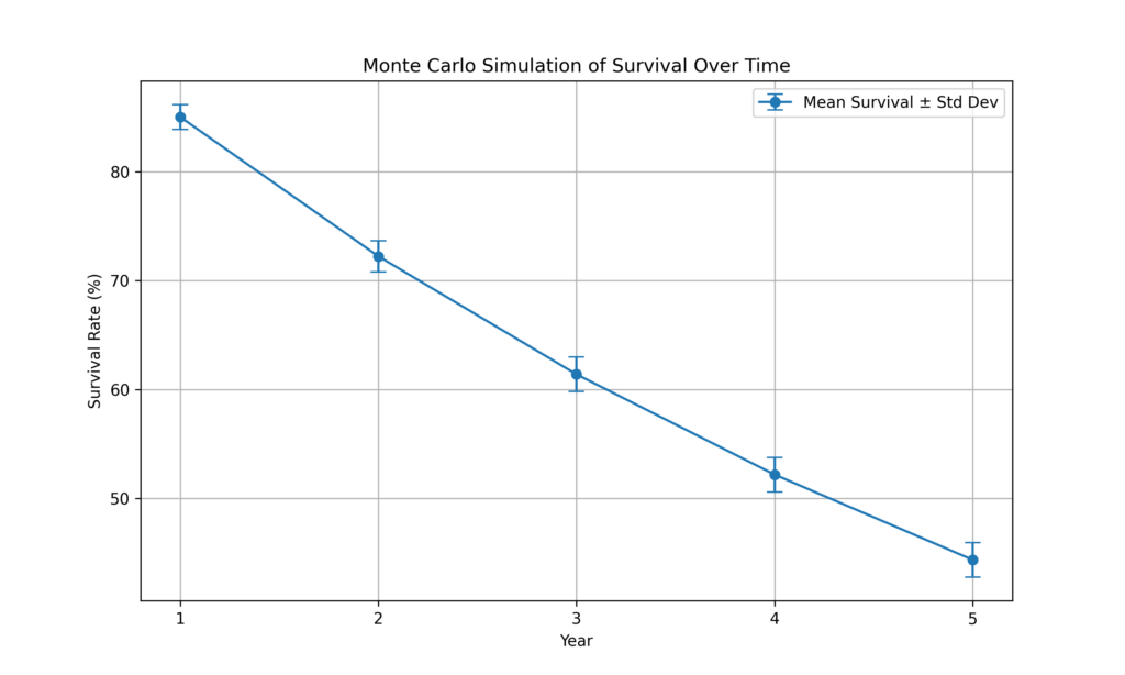
Step 4: visualize results

plt.figure(figsize=(10, 6)) years = np.arange(1, num\_years + 1) plt.errorbar(years, mean\_survival, yerr=std\_survival, fmt=’-o’, capsize=5, label=’Mean Survival ± Std Dev’) plt.title(‘Monte Carlo Simulation of Survival Over Time’) plt.xlabel(‘Year’) plt.ylabel(‘Survival Rate (%)’) plt.xticks(years) plt.grid(True) plt.legend() plt.show() ```
<span class="line"><span style="color: #F8F8F2">plt.figure(</span><span style="color: #FFB86C; font-style: italic">figsize</span><span style="color: #FF79C6">=</span><span style="color: #F8F8F2">(</span><span style="color: #BD93F9">10</span><span style="color: #F8F8F2">, </span><span style="color: #BD93F9">6</span><span style="color: #F8F8F2">))</span></span>
<span class="line"><span style="color: #F8F8F2">years </span><span style="color: #FF79C6">=</span><span style="color: #F8F8F2"> np.arange(</span><span style="color: #BD93F9">1</span><span style="color: #F8F8F2">, num_years </span><span style="color: #FF79C6">+</span><span style="color: #F8F8F2"> </span><span style="color: #BD93F9">1</span><span style="color: #F8F8F2">)</span></span>
<span class="line"><span style="color: #F8F8F2">plt.errorbar(years, mean_survival, </span><span style="color: #FFB86C; font-style: italic">yerr</span><span style="color: #FF79C6">=</span><span style="color: #F8F8F2">std_survival, </span><span style="color: #FFB86C; font-style: italic">fmt</span><span style="color: #FF79C6">=</span><span style="color: #E9F284">'</span><span style="color: #F1FA8C">-o</span><span style="color: #E9F284">'</span><span style="color: #F8F8F2">, </span><span style="color: #FFB86C; font-style: italic">capsize</span><span style="color: #FF79C6">=</span><span style="color: #BD93F9">5</span><span style="color: #F8F8F2">, </span><span style="color: #FFB86C; font-style: italic">label</span><span style="color: #FF79C6">=</span><span style="color: #E9F284">'</span><span style="color: #F1FA8C">Mean Survival ± Std Dev</span><span style="color: #E9F284">'</span><span style="color: #F8F8F2">)</span></span>
<span class="line"><span style="color: #F8F8F2">plt.title(</span><span style="color: #E9F284">'</span><span style="color: #F1FA8C">Monte Carlo Simulation of Survival Over Time</span><span style="color: #E9F284">'</span><span style="color: #F8F8F2">)</span></span>
<span class="line"><span style="color: #F8F8F2">plt.xlabel(</span><span style="color: #E9F284">'</span><span style="color: #F1FA8C">Year</span><span style="color: #E9F284">'</span><span style="color: #F8F8F2">)</span></span>
<span class="line"><span style="color: #F8F8F2">plt.ylabel(</span><span style="color: #E9F284">'</span><span style="color: #F1FA8C">Survival Rate (%)</span><span style="color: #E9F284">'</span><span style="color: #F8F8F2">)</span></span>
<span class="line"><span style="color: #F8F8F2">plt.xticks(years)</span></span>
<span class="line"><span style="color: #F8F8F2">plt.grid(</span><span style="color: #BD93F9">True</span><span style="color: #F8F8F2">)</span></span>
<span class="line"><span style="color: #F8F8F2">plt.legend()</span></span>
<span class="line"><span style="color: #F8F8F2">plt.show()</span></span>
<span class="line"></span>
```

![Monte Carlo simulation of Survival over time](https://www.micheledpierri.com/wp-content/uploads/2025/01/montecarlo1_0-1024x614.png)

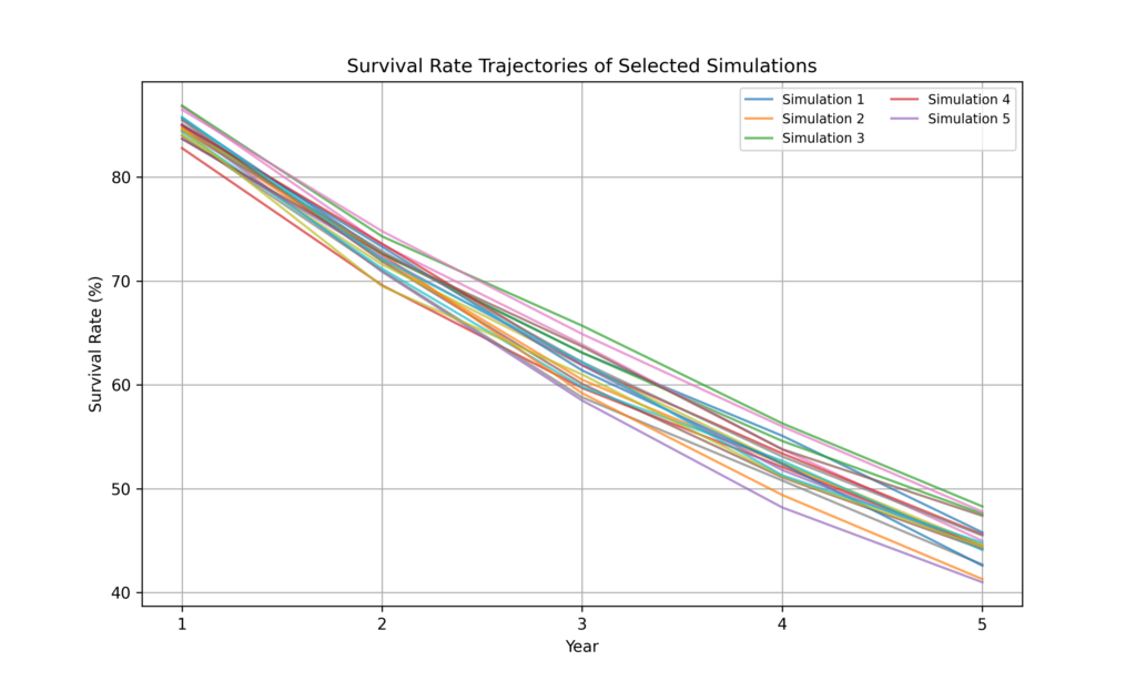
Step 4: visualize survival trajectories of a subset of simulations

plt.figure(figsize=(10, 6)) for i in range(20): # Plot trajectories for 20 random simulations plt.plot(years, survival\_data\[i, :\], alpha=0.7, label=f’Simulation {i+1}’ if i < 5 else “”) plt.title(‘Survival Rate Trajectories of Selected Simulations’) plt.xlabel(‘Year’) plt.ylabel(‘Survival Rate (%)’) plt.xticks(years) plt.grid(True) plt.legend(loc=’upper right’, fontsize=’small’, ncol=2, frameon=True) plt.show() ```
<span class="line"><span style="color: #F8F8F2">plt.figure(</span><span style="color: #FFB86C; font-style: italic">figsize</span><span style="color: #FF79C6">=</span><span style="color: #F8F8F2">(</span><span style="color: #BD93F9">10</span><span style="color: #F8F8F2">, </span><span style="color: #BD93F9">6</span><span style="color: #F8F8F2">))</span></span>
<span class="line"><span style="color: #FF79C6">for</span><span style="color: #F8F8F2"> i </span><span style="color: #FF79C6">in</span><span style="color: #F8F8F2"> </span><span style="color: #8BE9FD">range</span><span style="color: #F8F8F2">(</span><span style="color: #BD93F9">20</span><span style="color: #F8F8F2">):  </span><span style="color: #6272A4"># Plot trajectories for 20 random simulations</span></span>
<span class="line"><span style="color: #F8F8F2">    plt.plot(years, survival_data[i, </span><span style="color: #FF79C6">:</span><span style="color: #F8F8F2">], </span><span style="color: #FFB86C; font-style: italic">alpha</span><span style="color: #FF79C6">=</span><span style="color: #BD93F9">0.7</span><span style="color: #F8F8F2">, </span><span style="color: #FFB86C; font-style: italic">label</span><span style="color: #FF79C6">=</span><span style="color: #FF79C6">f</span><span style="color: #F1FA8C">'Simulation </span><span style="color: #BD93F9">{</span><span style="color: #F8F8F2">i</span><span style="color: #FF79C6">+</span><span style="color: #BD93F9">1}</span><span style="color: #F1FA8C">'</span><span style="color: #F8F8F2"> </span><span style="color: #FF79C6">if</span><span style="color: #F8F8F2"> i </span><span style="color: #FF79C6"><</span><span style="color: #F8F8F2"> </span><span style="color: #BD93F9">5</span><span style="color: #F8F8F2"> </span><span style="color: #FF79C6">else</span><span style="color: #F8F8F2"> </span><span style="color: #E9F284">""</span><span style="color: #F8F8F2">)</span></span>
<span class="line"><span style="color: #F8F8F2">plt.title(</span><span style="color: #E9F284">'</span><span style="color: #F1FA8C">Survival Rate Trajectories of Selected Simulations</span><span style="color: #E9F284">'</span><span style="color: #F8F8F2">)</span></span>
<span class="line"><span style="color: #F8F8F2">plt.xlabel(</span><span style="color: #E9F284">'</span><span style="color: #F1FA8C">Year</span><span style="color: #E9F284">'</span><span style="color: #F8F8F2">)</span></span>
<span class="line"><span style="color: #F8F8F2">plt.ylabel(</span><span style="color: #E9F284">'</span><span style="color: #F1FA8C">Survival Rate (%)</span><span style="color: #E9F284">'</span><span style="color: #F8F8F2">)</span></span>
<span class="line"><span style="color: #F8F8F2">plt.xticks(years)</span></span>
<span class="line"><span style="color: #F8F8F2">plt.grid(</span><span style="color: #BD93F9">True</span><span style="color: #F8F8F2">)</span></span>
<span class="line"><span style="color: #F8F8F2">plt.legend(</span><span style="color: #FFB86C; font-style: italic">loc</span><span style="color: #FF79C6">=</span><span style="color: #E9F284">'</span><span style="color: #F1FA8C">upper right</span><span style="color: #E9F284">'</span><span style="color: #F8F8F2">, </span><span style="color: #FFB86C; font-style: italic">fontsize</span><span style="color: #FF79C6">=</span><span style="color: #E9F284">'</span><span style="color: #F1FA8C">small</span><span style="color: #E9F284">'</span><span style="color: #F8F8F2">, </span><span style="color: #FFB86C; font-style: italic">ncol</span><span style="color: #FF79C6">=</span><span style="color: #BD93F9">2</span><span style="color: #F8F8F2">, </span><span style="color: #FFB86C; font-style: italic">frameon</span><span style="color: #FF79C6">=</span><span style="color: #BD93F9">True</span><span style="color: #F8F8F2">)</span></span>
<span class="line"><span style="color: #F8F8F2">plt.show()</span></span>
<span class="line"></span>
```

![Survival rate trajectories of selected simulations](https://www.micheledpierri.com/wp-content/uploads/2025/01/montecarlo1_1-1024x614.png)

## Example 2: Monte Carlo Simulation and Linear Regression

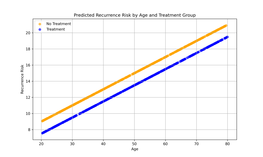
This example simulates the risk of recurrence using a linear regression model. The goal is to demonstrate how Monte Carlo simulation can be applied to assess the variability and confidence in predictions based on a linear regression model.

The risk of recurrence is evaluated using two independent variables: age (a continuous variable) and treatment status (a binary variable).

Required Python Libraries

import numpy as np import matplotlib.pyplot as plt import pandas as pd ```
<span class="line"><span style="color: #FF79C6">import</span><span style="color: #F8F8F2"> numpy </span><span style="color: #FF79C6">as</span><span style="color: #F8F8F2"> np</span></span>
<span class="line"><span style="color: #FF79C6">import</span><span style="color: #F8F8F2"> matplotlib.pyplot </span><span style="color: #FF79C6">as</span><span style="color: #F8F8F2"> plt</span></span>
<span class="line"><span style="color: #FF79C6">import</span><span style="color: #F8F8F2"> pandas </span><span style="color: #FF79C6">as</span><span style="color: #F8F8F2"> pd</span></span>
<span class="line"></span>
```

Step 1: define the parameters of simulation

np.random.seed(42) # Seed for reproducibility num\_patients = 1000 # Number of patients in the simulation num\_simulations = 1000 # Number of Monte Carlo iterations # Parameters for the linear regression model # True coefficients (for simulation purposes) beta\_0 = 5 # Intercept beta\_1 = 0.2 # Coefficient for age beta\_2 = -1.5 # Coefficient for treatment (binary: 0 or 1) sigma = 2 # Standard deviation of the noise term # Generate patient data ages = np.random.uniform(20, 80, num\_patients) # Ages uniformly distributed between 20 and 80 treatment = np.random.choice(\[0, 1\], size=num\_patients) # Random assignment to treatment groups (0 or 1) ```
<span class="line"><span style="color: #F8F8F2">np.random.seed(</span><span style="color: #BD93F9">42</span><span style="color: #F8F8F2">)  </span><span style="color: #6272A4"># Seed for reproducibility</span></span>
<span class="line"><span style="color: #F8F8F2">num_patients </span><span style="color: #FF79C6">=</span><span style="color: #F8F8F2"> </span><span style="color: #BD93F9">1000</span><span style="color: #F8F8F2">  </span><span style="color: #6272A4"># Number of patients in the simulation</span></span>
<span class="line"><span style="color: #F8F8F2">num_simulations </span><span style="color: #FF79C6">=</span><span style="color: #F8F8F2"> </span><span style="color: #BD93F9">1000</span><span style="color: #F8F8F2">  </span><span style="color: #6272A4"># Number of Monte Carlo iterations</span></span>
<span class="line"></span>
<span class="line"><span style="color: #6272A4"># Parameters for the linear regression model</span></span>
<span class="line"><span style="color: #6272A4"># True coefficients (for simulation purposes)</span></span>
<span class="line"><span style="color: #F8F8F2">beta_0 </span><span style="color: #FF79C6">=</span><span style="color: #F8F8F2"> </span><span style="color: #BD93F9">5</span><span style="color: #F8F8F2">  </span><span style="color: #6272A4"># Intercept</span></span>
<span class="line"><span style="color: #F8F8F2">beta_1 </span><span style="color: #FF79C6">=</span><span style="color: #F8F8F2"> </span><span style="color: #BD93F9">0.2</span><span style="color: #F8F8F2">  </span><span style="color: #6272A4"># Coefficient for age</span></span>
<span class="line"><span style="color: #F8F8F2">beta_2 </span><span style="color: #FF79C6">=</span><span style="color: #F8F8F2"> </span><span style="color: #FF79C6">-</span><span style="color: #BD93F9">1.5</span><span style="color: #F8F8F2">  </span><span style="color: #6272A4"># Coefficient for treatment (binary: 0 or 1)</span></span>
<span class="line"><span style="color: #F8F8F2">sigma </span><span style="color: #FF79C6">=</span><span style="color: #F8F8F2"> </span><span style="color: #BD93F9">2</span><span style="color: #F8F8F2">  </span><span style="color: #6272A4"># Standard deviation of the noise term</span></span>
<span class="line"></span>
<span class="line"><span style="color: #6272A4"># Generate patient data</span></span>
<span class="line"><span style="color: #F8F8F2">ages </span><span style="color: #FF79C6">=</span><span style="color: #F8F8F2"> np.random.uniform(</span><span style="color: #BD93F9">20</span><span style="color: #F8F8F2">, </span><span style="color: #BD93F9">80</span><span style="color: #F8F8F2">, num_patients)  </span><span style="color: #6272A4"># Ages uniformly distributed between 20 and 80</span></span>
<span class="line"><span style="color: #F8F8F2">treatment </span><span style="color: #FF79C6">=</span><span style="color: #F8F8F2"> np.random.choice([</span><span style="color: #BD93F9">0</span><span style="color: #F8F8F2">, </span><span style="color: #BD93F9">1</span><span style="color: #F8F8F2">], </span><span style="color: #FFB86C; font-style: italic">size</span><span style="color: #FF79C6">=</span><span style="color: #F8F8F2">num_patients)  </span><span style="color: #6272A4"># Random assignment to treatment groups (0 or 1)</span></span>
<span class="line"></span>
```

Step 2: runs the regression model multiple time with generated data

predicted\_risks = np.zeros((num\_simulations, num\_patients)) for sim in range(num\_simulations): # Generate recurrence risk with noise noise = np.random.normal(0, sigma, num\_patients) true\_risk = beta\_0 + beta\_1 \* ages + beta\_2 \* treatment + noise # Fit a linear regression model to the simulated data # (For simplicity, we assume the same predictors for all simulations) X = np.column\_stack((np.ones(num\_patients), ages, treatment)) # Design matrix beta\_hat = np.linalg.inv(X.T @ X) @ X.T @ true\_risk # Ordinary Least Squares estimate # Predict recurrence risk using the fitted model predicted\_risks\[sim, :\] = X @ beta\_hat ```
<span class="line"><span style="color: #F8F8F2">predicted_risks </span><span style="color: #FF79C6">=</span><span style="color: #F8F8F2"> np.zeros((num_simulations, num_patients))</span></span>
<span class="line"></span>
<span class="line"><span style="color: #FF79C6">for</span><span style="color: #F8F8F2"> sim </span><span style="color: #FF79C6">in</span><span style="color: #F8F8F2"> </span><span style="color: #8BE9FD">range</span><span style="color: #F8F8F2">(num_simulations):</span></span>
<span class="line"><span style="color: #F8F8F2">    </span><span style="color: #6272A4"># Generate recurrence risk with noise</span></span>
<span class="line"><span style="color: #F8F8F2">    noise </span><span style="color: #FF79C6">=</span><span style="color: #F8F8F2"> np.random.normal(</span><span style="color: #BD93F9">0</span><span style="color: #F8F8F2">, sigma, num_patients)</span></span>
<span class="line"><span style="color: #F8F8F2">    true_risk </span><span style="color: #FF79C6">=</span><span style="color: #F8F8F2"> beta_0 </span><span style="color: #FF79C6">+</span><span style="color: #F8F8F2"> beta_1 </span><span style="color: #FF79C6">*</span><span style="color: #F8F8F2"> ages </span><span style="color: #FF79C6">+</span><span style="color: #F8F8F2"> beta_2 </span><span style="color: #FF79C6">*</span><span style="color: #F8F8F2"> treatment </span><span style="color: #FF79C6">+</span><span style="color: #F8F8F2"> noise</span></span>
<span class="line"></span>
<span class="line"><span style="color: #F8F8F2">    </span><span style="color: #6272A4"># Fit a linear regression model to the simulated data</span></span>
<span class="line"><span style="color: #F8F8F2">    </span><span style="color: #6272A4"># (For simplicity, we assume the same predictors for all simulations)</span></span>
<span class="line"><span style="color: #F8F8F2">    X </span><span style="color: #FF79C6">=</span><span style="color: #F8F8F2"> np.column_stack((np.ones(num_patients), ages, treatment))  </span><span style="color: #6272A4"># Design matrix</span></span>
<span class="line"><span style="color: #F8F8F2">    beta_hat </span><span style="color: #FF79C6">=</span><span style="color: #F8F8F2"> np.linalg.inv(X.T </span><span style="color: #FF79C6">@</span><span style="color: #F8F8F2"> X) </span><span style="color: #FF79C6">@</span><span style="color: #F8F8F2"> X.T </span><span style="color: #FF79C6">@</span><span style="color: #F8F8F2"> true_risk  </span><span style="color: #6272A4"># Ordinary Least Squares estimate</span></span>
<span class="line"></span>
<span class="line"><span style="color: #F8F8F2">    </span><span style="color: #6272A4"># Predict recurrence risk using the fitted model</span></span>
<span class="line"><span style="color: #F8F8F2">    predicted_risks[sim, </span><span style="color: #FF79C6">:</span><span style="color: #F8F8F2">] </span><span style="color: #FF79C6">=</span><span style="color: #F8F8F2"> X </span><span style="color: #FF79C6">@</span><span style="color: #F8F8F2"> beta_hat</span></span>
<span class="line"></span>
```

Step 3 visualize the results with a plot of predicted risk against age for treatment and no treatment groups

plt.figure(figsize=(10, 6)) for treatment\_group in \[0, 1\]: group\_mask = (treatment == treatment\_group) label = ‘Treatment’ if treatment\_group == 1 else ‘No Treatment’ color = ‘blue’ if treatment\_group == 1 else ‘orange’ plt.scatter(ages\[group\_mask\], mean\_risk\[group\_mask\], alpha=0.6, label=label, color=color) plt.fill\_between( ages\[group\_mask\], mean\_risk\[group\_mask\] – std\_risk\[group\_mask\], mean\_risk\[group\_mask\] + std\_risk\[group\_mask\], color=color, alpha=0.3 ) plt.title(‘Predicted Recurrence Risk by Age and Treatment Group’) plt.xlabel(‘Age’) plt.ylabel(‘Recurrence Risk’) plt.grid(True) plt.legend() plt.show() ```
<span class="line"><span style="color: #F8F8F2">plt.figure(</span><span style="color: #FFB86C; font-style: italic">figsize</span><span style="color: #FF79C6">=</span><span style="color: #F8F8F2">(</span><span style="color: #BD93F9">10</span><span style="color: #F8F8F2">, </span><span style="color: #BD93F9">6</span><span style="color: #F8F8F2">))</span></span>
<span class="line"><span style="color: #FF79C6">for</span><span style="color: #F8F8F2"> treatment_group </span><span style="color: #FF79C6">in</span><span style="color: #F8F8F2"> [</span><span style="color: #BD93F9">0</span><span style="color: #F8F8F2">, </span><span style="color: #BD93F9">1</span><span style="color: #F8F8F2">]:</span></span>
<span class="line"><span style="color: #F8F8F2">    group_mask </span><span style="color: #FF79C6">=</span><span style="color: #F8F8F2"> (treatment </span><span style="color: #FF79C6">==</span><span style="color: #F8F8F2"> treatment_group)</span></span>
<span class="line"><span style="color: #F8F8F2">    label </span><span style="color: #FF79C6">=</span><span style="color: #F8F8F2"> </span><span style="color: #E9F284">'</span><span style="color: #F1FA8C">Treatment</span><span style="color: #E9F284">'</span><span style="color: #F8F8F2"> </span><span style="color: #FF79C6">if</span><span style="color: #F8F8F2"> treatment_group </span><span style="color: #FF79C6">==</span><span style="color: #F8F8F2"> </span><span style="color: #BD93F9">1</span><span style="color: #F8F8F2"> </span><span style="color: #FF79C6">else</span><span style="color: #F8F8F2"> </span><span style="color: #E9F284">'</span><span style="color: #F1FA8C">No Treatment</span><span style="color: #E9F284">'</span></span>
<span class="line"><span style="color: #F8F8F2">    color </span><span style="color: #FF79C6">=</span><span style="color: #F8F8F2"> </span><span style="color: #E9F284">'</span><span style="color: #F1FA8C">blue</span><span style="color: #E9F284">'</span><span style="color: #F8F8F2"> </span><span style="color: #FF79C6">if</span><span style="color: #F8F8F2"> treatment_group </span><span style="color: #FF79C6">==</span><span style="color: #F8F8F2"> </span><span style="color: #BD93F9">1</span><span style="color: #F8F8F2"> </span><span style="color: #FF79C6">else</span><span style="color: #F8F8F2"> </span><span style="color: #E9F284">'</span><span style="color: #F1FA8C">orange</span><span style="color: #E9F284">'</span></span>
<span class="line"><span style="color: #F8F8F2">    plt.scatter(ages[group_mask], mean_risk[group_mask], </span><span style="color: #FFB86C; font-style: italic">alpha</span><span style="color: #FF79C6">=</span><span style="color: #BD93F9">0.6</span><span style="color: #F8F8F2">, </span><span style="color: #FFB86C; font-style: italic">label</span><span style="color: #FF79C6">=</span><span style="color: #F8F8F2">label, </span><span style="color: #FFB86C; font-style: italic">color</span><span style="color: #FF79C6">=</span><span style="color: #F8F8F2">color)</span></span>
<span class="line"><span style="color: #F8F8F2">    plt.fill_between(</span></span>
<span class="line"><span style="color: #F8F8F2">        ages[group_mask],</span></span>
<span class="line"><span style="color: #F8F8F2">        mean_risk[group_mask] </span><span style="color: #FF79C6">-</span><span style="color: #F8F8F2"> std_risk[group_mask],</span></span>
<span class="line"><span style="color: #F8F8F2">        mean_risk[group_mask] </span><span style="color: #FF79C6">+</span><span style="color: #F8F8F2"> std_risk[group_mask],</span></span>
<span class="line"><span style="color: #F8F8F2">        </span><span style="color: #FFB86C; font-style: italic">color</span><span style="color: #FF79C6">=</span><span style="color: #F8F8F2">color, </span><span style="color: #FFB86C; font-style: italic">alpha</span><span style="color: #FF79C6">=</span><span style="color: #BD93F9">0.3</span></span>
<span class="line"><span style="color: #F8F8F2">    )</span></span>
<span class="line"></span>
<span class="line"><span style="color: #F8F8F2">plt.title(</span><span style="color: #E9F284">'</span><span style="color: #F1FA8C">Predicted Recurrence Risk by Age and Treatment Group</span><span style="color: #E9F284">'</span><span style="color: #F8F8F2">)</span></span>
<span class="line"><span style="color: #F8F8F2">plt.xlabel(</span><span style="color: #E9F284">'</span><span style="color: #F1FA8C">Age</span><span style="color: #E9F284">'</span><span style="color: #F8F8F2">)</span></span>
<span class="line"><span style="color: #F8F8F2">plt.ylabel(</span><span style="color: #E9F284">'</span><span style="color: #F1FA8C">Recurrence Risk</span><span style="color: #E9F284">'</span><span style="color: #F8F8F2">)</span></span>
<span class="line"><span style="color: #F8F8F2">plt.grid(</span><span style="color: #BD93F9">True</span><span style="color: #F8F8F2">)</span></span>
<span class="line"><span style="color: #F8F8F2">plt.legend()</span></span>
<span class="line"><span style="color: #F8F8F2">plt.show()</span></span>
<span class="line"></span>
```

![Predicted recurrence risk by age and treatment froup](https://www.micheledpierri.com/wp-content/uploads/2025/01/montecarlo2_0-1024x614.png)

## Conclusion

Monte Carlo simulation is a powerful tool that enables modeling, analyzing, and optimizing clinical studies when faced with uncertainty. It provides a robust foundation for improving study design, supporting clinical and regulatory decisions, and predicting long-term outcomes. However, its effectiveness depends on the quality of underlying assumptions.