---
title: Survival Analysis
date: 2025-11-17T16:24:52Z
modified: 2026-07-20T19:32:28Z
permalink: "https://www.micheledpierri.com/statistics/survival-analysis/"
type: page
status: publish
excerpt: ""
wpid: 2290
featured_image: "https://www.micheledpierri.com/wp-content/uploads/2026/07/st_survival_analysis_.png"
featured_image_alt: A long hospital ward in a vintage painterly style is engulfed in creeping darkness, with many occupied beds on the left; at the center, a patient, a nurse, a doctor, and other figures form a taut human chain across a deep chasm, linking the dying ward to a bright exit marked “Recovery.”
timestamp: 2026-07-20T19:32:28Z
tags: []
---
Survival Analysis is a statistical framework for studying the time until an event of interest occurs, such as death, relapse, reoperation, device failure, or hospital readmission.
Unlike standard regression methods, survival analysis explicitly accounts for **censoring**, **time-dependent risk**, and **non-Gaussian distributions**, making it essential for clinical research, biomedical engineering, and reliability studies.
This article provides a concise yet technically rigorous overview of the main concepts, mathematical foundations, dataset organization principles, and a practical Python workflow for Kaplan–Meier estimation, Cox regression, and survival curve interpretation.
**In brief**
- Survival analysis studies time‑to‑event data with censoring and time‑varying risk.
- Key functions: survival S(t), hazard h(t), cumulative hazard H(t) with S(t)=e^{-H(t)}.
- Kaplan–Meier estimates S(t). Nelson–Aalen estimates H(t).
- Cox PH models covariate effects via hazard ratios, assuming proportional hazards.
- Python workflow uses lifelines for KM, Cox, diagnostics, and plots with number‑at‑risk.
# ✅ **Introduction**
Survival analysis is used whenever we are interested not only in _whether_ an event happens, but _when_ it happens.
This applies to dozens of medical and scientific questions:
- How long do patients survive after surgery?
- How quickly do devices fail after implantation?
- When does cancer recur after treatment?
- How long do patients remain event-free during follow-up?
Unlike standard regression or classification problems, survival data have a unique property:
**not all events are observed**. Some patients reach the end of follow-up without experiencing the event, or they are lost to follow-up.
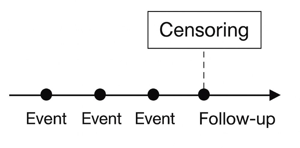
We do not want to discard these patients, because they still provide valuable information.
To deal with this, survival analysis uses a family of tools that:
1. correctly handle **partially observed outcomes** (censoring),
2. describe **how risk evolves over time**,
3. and allow us to study how predictors influence the **timing** of the event.
Before diving into mathematics, it is essential to build an intuitive mental model of how survival methods work.
Two ideas form the foundation of nearly everything in survival analysis:
- **Kaplan–Meier curves**, which describe _how many_ individuals remain event-free over time,
- **Cox proportional hazards models**, which describe _how predictors affect the risk_ of experiencing the event.
We start with these two concepts using intuition and visual reasoning, and only later introduce the mathematical objects behind them.
---
# ✅ **1. Kaplan–Meier: An Intuitive Explanation**
Imagine following 100 patients after a cardiac operation.
Every day, some patients may experience the event (e.g., death), while others remain alive; some may stop attending follow-up.
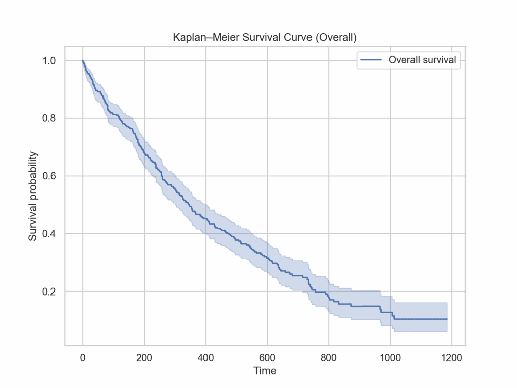
If we plot the count of patients who are still alive over time, we obtain a **stepwise survival curve**.
This is essentially what the **Kaplan–Meier estimator** does.
### **What problem does Kaplan–Meier solve?**
If we simply compute “percentage alive at 1 year”, we would have to exclude censored patients.
This wastes information.
Kaplan–Meier instead uses _all_ available follow-up:
- when an event occurs, the curve steps down,
- when a patient is censored, the curve stays flat but that person is no longer considered “at risk” afterwards.
This gives a **non-parametric summary** of survival over time that correctly accounts for incomplete follow-up.
### **How to read a Kaplan–Meier curve**
A KM curve answers:
- _What proportion of the cohort is still event-free at time ttt?_
- _When does the curve drop most steeply?_ (periods of higher risk)
- _What is the median survival?_ (the time when survival reaches 50%)
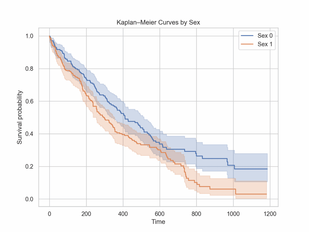
### **Comparing groups**
If we split patients by a factor — for example, diabetics vs non-diabetics — we can draw two KM curves:
- If the curves separate early → one group experiences events sooner.
- If the curves remain close → groups have similar survival.
- The log-rank test provides a statistical comparison of the curves.
### **Why is KM important?**
KM is the entry point to survival analysis because it:
- visualises the survival experience of the cohort,
- handles censored data naturally,
- reveals temporal patterns (early vs late risk),
- provides clinical intuition before modelling.
It is descriptive, not inferential.
It tells us **what happens**, not **why**.
To understand _why_ some patients have higher risk, we need a model.
---
# ✅ **2. Cox Proportional Hazards: An Intuitive Explanation**
While Kaplan–Meier describes survival _without_ accounting for predictors, the **Cox proportional hazards model** explains _how predictors modify the risk over time_.
### **The key idea**
Cox does not try to predict the “exact survival time”.
Instead, it compares individuals who are **at risk at the same moment**, and quantifies how much more (or less) likely one patient is to experience the event compared to another.
This comparison produces the **hazard ratio (HR)**.
### **What is the hazard ratio? (Intuition)**
If two patients are identical except for one characteristic:
- HR = 2 → one patient has _twice the instantaneous risk_ of experiencing the event at any time
- HR = 0.5 → one patient has _half the instantaneous risk_
- HR = 1 → no difference
Importantly:
- The Cox model does _not_ assume anything about the shape of the baseline risk over time. Early risk, late risk, U-shaped risk — all allowed.
- It only assumes that the _ratio_ between risks of two individuals stays constant over time. This is the **proportional hazards assumption**.
### **Why Cox is powerful**
Cox allows us to:
- quantify the effect of continuous predictors (age, creatinine, EuroSCORE II),
- adjust for multiple risk factors simultaneously,
- estimate adjusted survival curves for selected profiles,
- test whether predictors violate proportionality (Schoenfeld residuals).
### **What Cox does _not_ do**
- It does not estimate absolute survival probability without additional steps.
- It does not assume a distribution (e.g., exponential, Weibull).
- It does not tell you the baseline hazard explicitly (though it can be estimated).
### **KM vs Cox: intuition**
| Goal | Method |
| --- | --- |
| How many patients survive over time? | Kaplan–Meier |
| Do groups differ in unadjusted survival? | Kaplan–Meier + log-rank |
| How do multiple predictors affect risk? | Cox model |
| How does risk accumulate? | Nelson–Aalen |
Having built an intuitive understanding of how survival curves and hazard ratios work, we can now formalize these ideas using their underlying mathematical functions.
---
# ✅ Mathematical Foundations of Survival Analysis
Survival analysis relies on mathematical functions that describe time-to-event data. Understanding these interconnected functions is essential for interpreting survival curves, hazards, and Cox models.
## Time-to-Event Variable
Let:
![\[T \ge 0\]](https://www.micheledpierri.com/wp-content/ql-cache/quicklatex.com-33b73a0747b6cf1ffabda718b8aab8bd_l3.svg "Rendered by QuickLaTeX.com")
be a **non-negative random variable** representing the time until the event of interest (death, relapse, reoperation, etc.).
- T = 0 represents the time origin (baseline: surgery, diagnosis, randomization).
- T = t represents the time the event occurs.
## Distribution Function and Density
### Cumulative Distribution Function (CDF)
![\[F(t) = \Pr(T \le t)\]](https://www.micheledpierri.com/wp-content/ql-cache/quicklatex.com-be7377709d7cffd998b224f3f6838e80_l3.svg "Rendered by QuickLaTeX.com")
- Represents the **probability that the event has occurred by time t**.
- It is a non-decreasing function, starting at 0 and converging to 1 (if all eventually experience the event).
### Probability Density Function (PDF)
If T is continuous, it admits a density:
![\[f(t) = \frac{dF(t)}{dt}\]](https://www.micheledpierri.com/wp-content/ql-cache/quicklatex.com-8e7f1180ad00551b57a31e8967d8e974_l3.svg "Rendered by QuickLaTeX.com")
- Represents the **instantaneous accumulation rate** of event probability around time t.
- It is not itself a probability, but integrates to 1.
### Survival Function
The survival function is the central object of survival analysis:
![\[S(t) = \Pr(T > t)\]](https://www.micheledpierri.com/wp-content/ql-cache/quicklatex.com-6c63e9124cff3c69d064618cef9d4504_l3.svg "Rendered by QuickLaTeX.com")
This means:
- The probability that an individual **survives beyond time t** without experiencing the event.
- It is a **non-increasing** function:
- S(0) = 1 (everyone is alive at time zero),
- S(t) to 0 as t to infinity (if the event is certain),
- flatter curves → better survival.
Relationship with the CDF:
![\[S(t) = 1 - F(t)\]](https://www.micheledpierri.com/wp-content/ql-cache/quicklatex.com-83a8bbb2fcd9e0e63ce53bf1366e8e34_l3.svg "Rendered by QuickLaTeX.com")
### Hazard Function (Instantaneous Risk)
The hazard function describes the **instantaneous risk of experiencing the event at time t**, given survival up to that time.
![\[h(t) = \lim_{\Delta t\to 0} \frac{\Pr(t \le T < t + \Delta t \mid T \ge t)}{\Delta t}\]](https://www.micheledpierri.com/wp-content/ql-cache/quicklatex.com-250ebb75a202637fa3e8573316ebf553_l3.svg "Rendered by QuickLaTeX.com")
Interpretation:
- It is **not a probability**: hazards can exceed 1.
- It measures **how dangerous the moment t is** for someone who has survived up to t.
- High hazard at t: steep drop in survival curve at t.
Relationship with the PDF and survival function:
![\[h(t) = \frac{f(t)}{S(t)}\]](https://www.micheledpierri.com/wp-content/ql-cache/quicklatex.com-1e68aad387e856e31ecb777e020922e6_l3.svg "Rendered by QuickLaTeX.com")
Meaning:
- The instantaneous density of events divided by the probability of still being at risk.
### Cumulative Hazard Function
Defined as:
![\[H(t) = \int_0^t h(u)\,du\]](https://www.micheledpierri.com/wp-content/ql-cache/quicklatex.com-c1a5baf5c8f8fea6d2ce32585d1a5391_l3.svg "Rendered by QuickLaTeX.com")
- Aggregates the total hazard accumulated up to time t.
- It is a **non-decreasing** function.
- Has a key link to survival:
![\[S(t) = \exp[-H(t)]\]](https://www.micheledpierri.com/wp-content/ql-cache/quicklatex.com-5d14fb26e87c3385c75233646c709569_l3.svg "Rendered by QuickLaTeX.com")
Meaning:
- Survival decreases exponentially with cumulative hazard.
### Relationship Between Survival and Hazard
Because the hazard, survival, density, and cumulative hazard all derive from one another, we can express them interchangeably. For instance:
![\[H(t) = \int_0^t \frac{f(u)}{S(u)}\,du\]](https://www.micheledpierri.com/wp-content/ql-cache/quicklatex.com-21a91157af4894776995871f4c114ada_l3.svg "Rendered by QuickLaTeX.com")
This expresses the cumulative hazard in terms of the PDF and survival.
### Median Survival Time
The median survival time is the earliest time at which the survival function drops to 0.5:
![\[\text{Median survival} = \inf \{ t : S(t) \le 0.5 \}\]](https://www.micheledpierri.com/wp-content/ql-cache/quicklatex.com-ed9d91b5d7400a6ede0c0a323c1680f1_l3.svg "Rendered by QuickLaTeX.com")
This measure is robust and often preferred to the mean in right-skewed distributions.
### Cox Proportional Hazards Model
The Cox model relates survival time to covariates while leaving the baseline hazard unspecified:
![\[h(t \mid X_i) = h_0(t)\exp(\beta_1 X_{i1} + \beta_2 X_{i2} + \dots + \beta_p X_{ip})\]](https://www.micheledpierri.com/wp-content/ql-cache/quicklatex.com-99a23f939ed3f2ae201353c12ad4e70e_l3.svg "Rendered by QuickLaTeX.com")
Here:
- h0(t) is the unspecified **baseline hazard**.
- β coefficients measure the effect of covariates on the hazard.
- Covariates may be binary (e.g., sex), continuous (e.g., age), or categorical.
The central quantity is the **hazard ratio (HR)**:
![\[\mathrm{HR} = \exp(\beta)\]](https://www.micheledpierri.com/wp-content/ql-cache/quicklatex.com-bdc6832cd33b8b54c8c00c4163c3cc2c_l3.svg "Rendered by QuickLaTeX.com")
Interpretation:
- HR > 1: increased hazard (worse prognosis).
- HR < 1: decreased hazard (protective).
- HR = 2: hazard doubled relative to baseline.
## Proportional Hazards Assumption
The defining assumption of the Cox model is that hazard ratios are constant over time. Formally:
![\[\frac{h(t \mid X_1)}{h(t \mid X_2)} = \exp\big[\beta^\top (X_1 - X_2)\big]\]](https://www.micheledpierri.com/wp-content/ql-cache/quicklatex.com-cd491bd378358d3a6c620f5ff348e752_l3.svg "Rendered by QuickLaTeX.com")
Meaning:
- The effect of covariates multiplies the hazard but does _not_ depend on time t.
- If hazards cross visibly in KM curves, the assumption is likely violated.
### Complete Cheat Sheet (All Formulas Together)
For convenience, here is a single block containing the full set of fundamental equations:
![\[\begin{aligned} T &\ge 0 \\ F(t) &= \Pr(T \le t) \\ f(t) &= \frac{dF(t)}{dt} \\ S(t) &= \Pr(T > t) = 1 - F(t) \\ h(t) &= \lim_{\Delta t\to 0} \frac{\Pr(t \le T < t + \Delta t \mid T \ge t)}{\Delta t} \\ h(t) &= \frac{f(t)}{S(t)} \\ H(t) &= \int_0^t h(u)\,du \\ S(t) &= \exp[-H(t)] \\ \text{Median survival} &= \inf \{ t : S(t) \le 0.5 \} \\ h(t \mid X) &= h_0(t)\exp(\beta^\top X) \\ \mathrm{HR} &= \exp(\beta) \end{aligned}\]](https://www.micheledpierri.com/wp-content/ql-cache/quicklatex.com-0ce3a01729db43e67602f54844356d95_l3.svg "Rendered by QuickLaTeX.com")
---
# ✅ **Nelson–Aalen: A Simple View of How Risk Accumulates Over Time**
While the Kaplan–Meier estimator describes _how many_ individuals remain event-free at each time point, the Nelson–Aalen estimator describes _how much risk has accumulated_ up to that moment.
It is the natural companion to Kaplan–Meier, but it looks at survival from the opposite direction.
Instead of asking:
> What is the probability of still being alive at time t?
the Nelson–Aalen estimator answers:
> How much hazard has the cohort accumulated by time ttt?
Every time an event occurs, the cumulative hazard increases by a small step.
If many patients experience the event while few remain at risk, the step is larger;
if the risk is low or no events occur, the curve stays flat.
This produces a **monotonic, stepwise curve** that grows whenever events happen and remains unchanged during event-free periods.
In practice:
- a **steep Nelson–Aalen curve** = a period of **high event intensity**,
- a **flat curve** = a **low-risk** interval.
Although clinicians tend to report Kaplan–Meier survival curves, Nelson–Aalen is essential behind the scenes: it forms the basis for estimating the **baseline hazard** in the Cox model and is useful for understanding _when_ the cohort faces elevated risk.
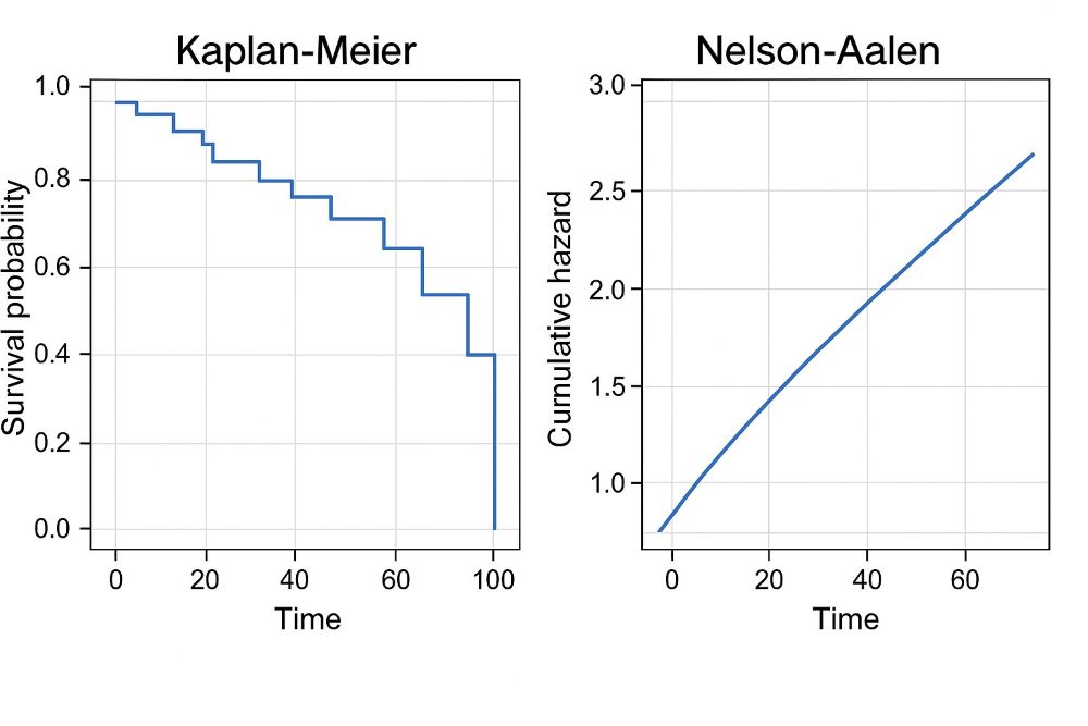
This cumulative-hazard perspective is also the foundation for estimating the Cox model’s baseline hazard, which explains why Nelson–Aalen and Cox are often presented together
---
# ✅Assumptions of Survival Analysis
A correct survival analysis depends critically on a small set of fundamental assumptions. If these assumptions are satisfied, survival estimates, hazard ratios, and model diagnostics have a clear interpretation. If they are violated, the results may become biased or misleading.
### Time Origin, Time Scale, and Follow-Up
Every survival model begins with a clear definition of time zero, because all subsequent assumptions depend on it.
Time zero may be:
- the date of surgery,
- the date of diagnosis,
- the date of randomization,
- the date of discharge.
Once the origin is fixed, every subject must have their follow-up measured consistently from that same moment. Likewise, the time scale (days, months, years) must be the same for all individuals.
If different patients effectively start counting from different types of events (e.g., some from diagnosis, others from treatment), even perfect statistical techniques will give distorted results, because the underlying timeline is inconsistent.
In short:
- A single, shared time origin
- A single, coherent time scale
- A consistent definition of follow-up
These form the foundation on which survival models can operate meaningfully.
### Event Observation and Censoring: What We Know About Each Patient
In survival data, two quantities are recorded for every subject:
- How long they were observed
- Whether they experienced the event or not
- If the event does not occur within the observation window, the observation is right-censored.
This leads to one of the most important assumptions of all survival models:
> Survival analysis assumes that the reason a subject becomes censored does not carry additional information about their underlying risk—beyond what is already measured in the dataset.
In other words, a censored patient should be statistically similar to a non-censored patient with the same covariates.
This assumption is satisfied when:
- the study ends for everyone at the same administrative date;
- patients miss follow-up for reasons unrelated to prognosis;
- the time of censoring is independent of the time of the event.
It is violated when:
- frail or critically ill patients systematically drop out earlier;
- healthier patients preferentially attend follow-up visits;
- loss to follow-up is correlated with the progression of disease.
If censoring is informative, Kaplan–Meier and Cox estimates tend to be biased, often in optimistic directions.
### Independence of Observations
Most classical survival methods assume that observations are independent:
- each row corresponds to a single subject,
- subjects do not influence each other’s risks.
In real data this assumption may fail:
- patients treated within the same hospital or by the same surgeon may share unmeasured characteristics;
- individuals in family or cluster settings may have correlated risks;
- repeated events within the same subject require specialized modeling.
When independence is doubtful, robust standard errors, frailty terms, or mixed-effects models may be appropriate.
In standard clinical datasets (e.g., single event per patient), independence is usually a reasonable working assumption.
### Assumptions for Kaplan–Meier Estimation
Kaplan–Meier is mathematically simple and robust. Its assumptions are:
1. Censoring is non-informative (as explained above).
2. Event times are precisely known (not interval-censored).
3. Observations are independent.
4. Competing risks are either absent or treated as censoring.
Note: when competing risks are substantial, Kaplan–Meier can overestimate the incidence of the event of interest. Use the Cumulative Incidence Function and, for regression, Fine–Gray models.
Quando queste condizioni tengono, la curva di Kaplan–Meier fornisce un quadro pulito e non distorto della sopravvivenza nel tempo.
### Assumption of the Cox Model
The Cox proportional hazards model introduces a major simplification:
it assumes that risk factors multiply the hazard by a constant factor that does not vary with time.
In other words:
- If a certain covariate doubles the hazard at day 30, it also doubles it at day 300 and at day 1000.
- The baseline hazard may change with time in any arbitrary way, but the effect of the covariates remains proportional across the entire timeline.
This is the Proportional Hazards (PH) assumption.
When PH holds, hazard ratios have a simple and intuitive interpretation.
When PH is violated (e.g., hazards cross visibly), Cox estimates may remain “statistically significant” but become scientifically misleading, because they represent an average of effects that change over time.
The Cox model also assumes that continuous covariates influence the log-hazard linearly.
For example:
- age is assumed to increase the log-hazard at a constant rate per year;
- creatinine is assumed to have a smooth, linear effect.
But biological processes are rarely linear.
When continuous covariates have nonlinear effects, analysts may need:
- splines,
- polynomial terms,
- piecewise transformations.
Correct functional form is critical; otherwise hazard ratios may misrepresent the underlying relationship.
In many clinical settings, important variables change over time (e.g., postoperative complications, treatment changes, biomarkers).
Standard Cox regression assumes:
- either these time-dependent influences are small,
- or they are unrelated to the predictors in the model.
When important time-varying confounders exist, the Cox model is misspecified and advanced methods are needed:
- extended Cox models with time-dependent covariates,
- joint models,
- marginal structural models.
### Summary of Assumptions
Instead of memorizing lists, the assumptions of survival analysis form a coherent logic:
- Define time correctly
- same time zero, same time scale.
- Observe follow-up consistently
- no informative censoring.
- Ensure independence or adjust for clustering
- independence is the default assumption.
- Use appropriate model assumptions
- Kaplan–Meier requires minimal assumptions.
- Cox additionally requires:
- proportional hazards,
- linearity of log-hazard,
- no major time-dependent confounding.
- Check assumptions diagnostically
- graphs, residuals, and tests help confirm model validity.
When these principles are respected, survival analysis provides reliable, interpretable, and clinically meaningful estimates of risk and prognosis.
---
# ✅ Dataset Organization for Survival Analysis
A robust survival analysis starts long before writing code. It starts with precise design of the dataset. Here we detail how to define variables, structure the data, and prepare them for Python.
## Core Variables: Time and Event
The two fundamental columns in any survival dataset are:
- **Duration variable (`time`, `follow_up`, etc.)**
- Represents the **time elapsed** between a clearly defined start and end:
- from surgery to death
- from diagnosis to relapse
- from discharge to readmission
- Must be **non-negative** and in a consistent unit (days, months, years).
- **Event indicator (`event`, `status`, etc.)**
- **Binary**:
- 1 = event occurred
- 0 = censored
- Must clearly reflect the event definition used in your study.
time: 365
event: 1 # death within 1 year
time: 540
event: 0 # alive at last follow-up (censored)```
time: 365
event: 1 # death within 1 year
time: 540
event: 0 # alive at last follow-up (censored)
```
## Dates vs. Durations
In clinical databases, you often start with **dates**, not durations:
- `date_surgery`
- `date_last_follow_up`
- `date_death` (if applicable)
You then derive:
- `time` = difference between two dates (e.g., days)
- `event` = 1 if death occurred before or at `date_last_follow_up`, 0 otherwise
Python example:
import pandas as pd
df = pd.read_csv("raw_clinical_data.csv", parse_dates=["date_surgery", "date_last_fu", "date_death"])
# duration in days from surgery to last observed time (death or last FU)
df["time"] = (df["date_last_fu"] - df["date_surgery"]).dt.days
# event = 1 if death date is not null and <= last follow-up, else 0
df["event"] = ((df["date_death"].notna()) &
(df["date_death"] <= df["date_last_fu"])).astype(int)```
import pandas as pd
df = pd.read_csv("raw_clinical_data.csv", parse_dates=["date_surgery", "date_last_fu", "date_death"])
# duration in days from surgery to last observed time (death or last FU)
df["time"] = (df["date_last_fu"] - df["date_surgery"]).dt.days
# event = 1 if death date is not null and <= last follow-up, else 0
df["event"] = ((df["date_death"].notna()) &
(df["date_death"] <= df["date_last_fu"])).astype(int)
```
This step is critical: any mistake in date handling will directly affect survival times and bias the analysis.
## Covariates: Types and Coding
Beyond `time` and `event`, your dataset typically includes **covariates** that may influence risk:
### 1. Continuous variables
Examples:
- `age` (years)
- `creatinine` (mg/dL)
- `left_ventricular_ejection_fraction`
Recommendations:
- Keep units clinically meaningful.
- Consider transformations when distributions are highly skewed (e.g., log(creatinine)).
### 2. Categorical variables
Examples:
- `sex` (male/female)
- `diabetes` (yes/no)
- `NYHA_class` (I, II, III, IV)
In Python and statistical modeling, these are typically converted into:
- **Binary indicators (dummy variables)** for each category (or all but one reference category). Example: `sex` → `sex_male` (1 = male, 0 = female as reference).
With `pandas` and `lifelines`, you can often pass categorical variables directly and let the library handle encoding, but explicit control is often preferable in clinical research.
### 3. Ordinal variables
Variables that have a natural order but not a precise numerical distance:
- `NYHA`
- `Killip class`
- `tumor_stage` (I–IV)
Options:
- Treat as **continuous** (if the scale is approximately linear in risk),
- Or convert to **dummy variables** (e.g., NYHA III–IV vs I–II),
- Or model with **splines** if risk increases non-linearly.
Explicitly justify your choice in a scientific context.
## Baseline vs Time-Dependent Covariates
In basic survival analysis, we often use **baseline covariates**:
- measured once at time zero (e.g., age, sex, preoperative risk scores).
However, some variables change over time:
- hemodynamic parameters,
- occurrence of complications,
- treatment changes,
- lab values.
If these time-varying variables are important, you need a **time-dependent survival dataset**, often in **long format**:
- One row per subject per time interval
- With updated covariate values
In this introductory lesson, we focus on **baseline-only models**.
## Wide vs Long Format Datasets
Two common structures:
- **Wide format** (most common in simple survival models)
- One row per patient
- Columns: `id`, `time`, `event`, `age`, `sex`, `bmi`, `euroscore`, etc.
- Suitable for:
- Kaplan–Meier
- Cox PH with baseline covariates
- **Long format**
- Multiple rows per patient
- Columns may include `start_time`, `end_time`, `event`, time-varying covariates
- Used for:
- time-dependent covariates,
- recurrent events,
- counting-process notation models.
For a first implementation with lifelines and standard Cox, wide format is usually sufficient.
## Handling Missing Data
As in any regression model, missing data can cause bias and loss of power.
Options:
- **Complete-case analysis** (exclude rows with missing covariates)
- Simple but may bias results if missingness is not completely at random.
- **Imputation** (e.g., multiple imputation)
- More advanced but statistically preferable in serious clinical research.
In the dataset used for survival analysis, you should:
1. Clearly document which variables have missing values.
2. Decide a strategy (e.g., complete-case for a tutorial, multiple imputation in publications).
3. Apply the same treatment across all models.
## Minimal Dataset for a First Python Survival Analysis
A minimal but realistic dataset for your Python scripts might include:
- `time`: follow-up in days from surgery to death/last contact
- `id`: patient identifier
- `event`: 1 if death occurred, 0 if censored
- `age`: at surgery
- `sex`: 0 = female, 1 = male
- `euroscore`: predicted risk at baseline (continuous)
- `bmi`: body mass index
- `diabetes`: 0/1
- `copd`: 0/1
- `creatinine`: mg/dL
In CSV:
id,time,event,age,sex,euroscore,bmi,diabetes,copd,creatinine
1,365,1,72,1,3.4,27,1,0,1.10
2,540,0,81,0,7.1,25,0,1,1.80
3,120,1,65,1,2.1,28,1,0,0.90
4,900,0,59,1,1.2,31,0,0,1.00
...```
id,time,event,age,sex,euroscore,bmi,diabetes,copd,creatinine
1,365,1,72,1,3.4,27,1,0,1.10
2,540,0,81,0,7.1,25,0,1,1.80
3,120,1,65,1,2.1,28,1,0,0.90
4,900,0,59,1,1.2,31,0,0,1.00
...
```
This structure is immediately compatible with `lifelines`:
import pandas as pd
from lifelines import CoxPHFitter
df = pd.read_csv("survival_data.csv")
# Fit Cox model with multiple covariates
cph = CoxPHFitter()
cph.fit(df, duration_col="time", event_col="event",
formula="age + sex + euroscore + bmi + diabetes + copd + creatinine")
cph.print_summary()```
import pandas as pd
from lifelines import CoxPHFitter
df = pd.read_csv("survival_data.csv")
# Fit Cox model with multiple covariates
cph = CoxPHFitter()
cph.fit(df, duration_col="time", event_col="event",
formula="age + sex + euroscore + bmi + diabetes + copd + creatinine")
cph.print_summary()
```
## Reproducible Workflow: Raw → Clean → Analysis
- **Raw data**
- Direct export from the hospital information system, registry, or database
- Contains dates, codes, free-text, missing or inconsistent entries
- **Clean analytic dataset for survival**
- Derived columns: `time`, `event`
- Well-defined covariates
- Clear handling of missing values
- Saved as `survival_analysis_dataset.csv`
- **Model-specific subsets**
- e.g., a version with only complete cases for Cox
- or a dataset restricted to a specific population (e.g., isolated CABG)
---
# ✅ Python Workflow: Scripts and Analysis
Importing libraries
import pandas as pd
from lifelines import KaplanMeierFitter, CoxPHFitter
from lifelines.plotting import add_at_risk_counts
import matplotlib.pyplot as plt```
import pandas as pd
from lifelines import KaplanMeierFitter, CoxPHFitter
from lifelines.plotting import add_at_risk_counts
import matplotlib.pyplot as plt
```
Loading and preparing the dataset
df = pd.read_csv("survival_data.csv")
# Ensure correct dtypes
df["event"] = df["event"].astype(int)
df["time"] = df["time"].astype(float)```
df = pd.read_csv("survival_data.csv")
# Ensure correct dtypes
df["event"] = df["event"].astype(int)
df["time"] = df["time"].astype(float)
```
Kaplan–Meier Estimator
km = KaplanMeierFitter()
km.fit(durations=df["time"], event_observed=df["event"])
fig, ax = plt.subplots(figsize=(8, 6))
km.plot_survival_function(ax=ax)
add_at_risk_counts(km, ax=ax)
plt.title("Kaplan–Meier Survival Curve")
plt.xlabel("Time (days)")
plt.ylabel("Survival Probability")
plt.tight_layout()
plt.show()```
km = KaplanMeierFitter()
km.fit(durations=df["time"], event_observed=df["event"])
fig, ax = plt.subplots(figsize=(8, 6))
km.plot_survival_function(ax=ax)
add_at_risk_counts(km, ax=ax)
plt.title("Kaplan–Meier Survival Curve")
plt.xlabel("Time (days)")
plt.ylabel("Survival Probability")
plt.tight_layout()
plt.show()
```
Cox Proportional Hazards Model
cph = CoxPHFitter()
cph.fit(df, duration_col="time", event_col="event")
cph.print_summary()```
cph = CoxPHFitter()
cph.fit(df, duration_col="time", event_col="event")
cph.print_summary()
```
Checking proportional hazards assumption
cph.check_assumptions(df, p_value_threshold=0.05)```
cph.check_assumptions(df, p_value_threshold=0.05)
```
## Interpretation of Results
### Kaplan–Meier
Look for:
- median survival time
- separation between strata (if groups are plotted)
- width of confidence intervals
- presence of early vs late risk
Interpretation example:
A steep early drop indicates a high early hazard (perioperative mortality), followed by plateau.
### Cox Model
Key parameters:
- **Hazard Ratio (HR)**:
- HR = exp(β) HR > 1 → increased risk; HR < 1 → protective effect.
- **p-value**: significance of covariate
- **95% CI**: uncertainty
- **Concordance (C-index)**: predictive accuracy
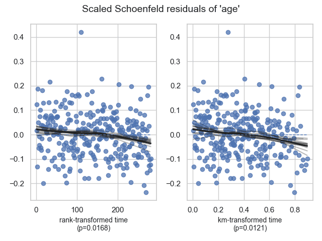
- **Schoenfeld test**: PH assumption check
Example interpretation:
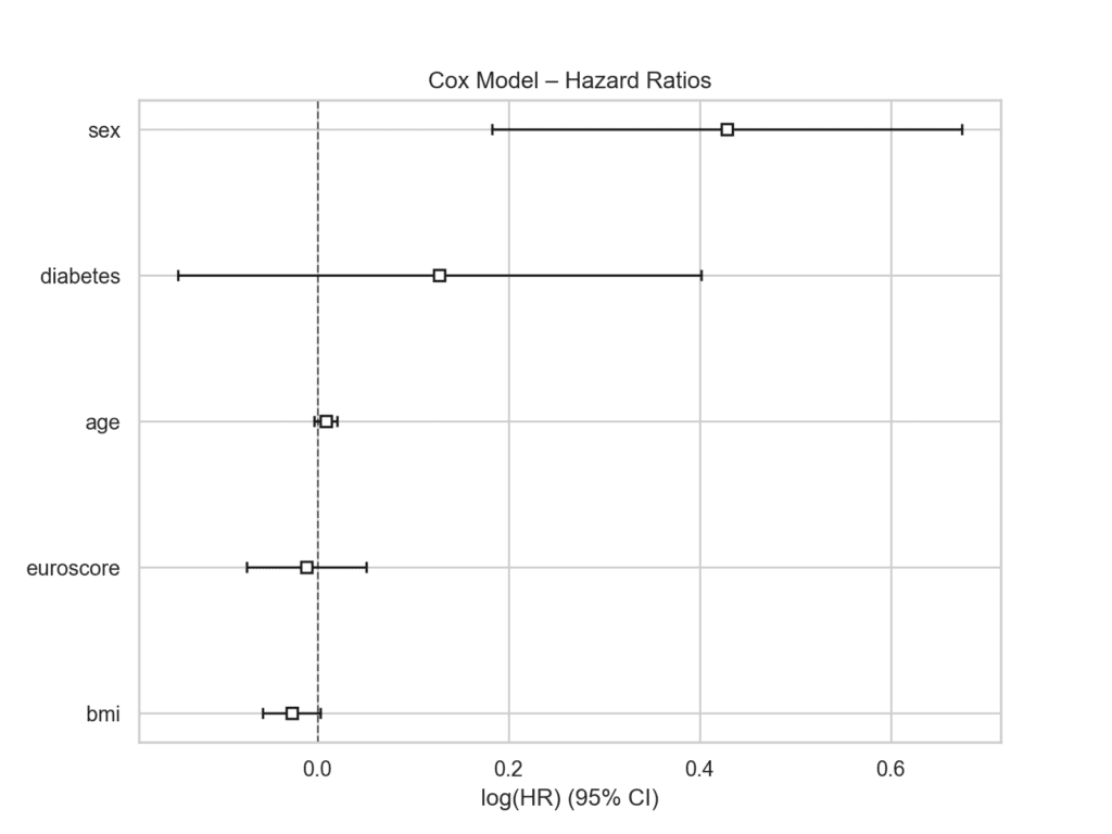
> Age (HR 1.04, p < 0.01) is a significant risk factor with a 4% increase in instantaneous mortality risk per year. EuroSCORE II demonstrates an expected positive association with hazard. BMI shows no significant effect.
## Graphical Outputs
### Kaplan–Meier Curves
- Survival function
- Confidence bands
- Number-at-risk table (optional)
### Cox Model Visualizations
- Forest plot of hazard ratios
- Schoenfeld residuals
---
# ✅ Complete Python Script – Survival Simulation + KM + Cox + Full Plots
"""
Survival Analysis Demo: Simulation + Kaplan–Meier + Cox PH Model
Author: Michele D. Pierri
This script creates a fully synthetic survival dataset, performs:
- Kaplan–Meier curves
- Stratified Kaplan–Meier curves
- Nelson–Aalen cumulative hazard
- Cox Proportional Hazards regression
- Model diagnostics (Schoenfeld residuals)
- Martingale & Deviance residual plots
with extremely verbose commentary for teaching purposes.
Libraries required:
pandas, numpy, lifelines, matplotlib, seaborn
"""
import numpy as np
import pandas as pd
import matplotlib.pyplot as plt
import seaborn as sns
from lifelines import KaplanMeierFitter, CoxPHFitter, NelsonAalenFitter
from lifelines.statistics import logrank_test
sns.set(style="whitegrid")
# ============================================================
# 1. Simulate a Survival Dataset
# ============================================================
# For reproducibility
np.random.seed(42)
N = 400 # number of subjects
# Continuous covariates
age = np.random.normal(loc=65, scale=10, size=N) # age in years
bmi = np.random.normal(loc=27, scale=4, size=N) # BMI
euroscore = np.clip(np.random.normal(3.5, 2.0, N), 0, 15) # simplified numeric risk score
# Binary covariates
sex = np.random.binomial(1, 0.60, N) # 1=male, 0=female
diabetes = np.random.binomial(1, 0.25, N)
# True hazard coefficients (for simulation only)
beta_age = 0.03 # hazard increases with age
beta_sex = 0.40 # males higher hazard
beta_diabetes = 0.60 # diabetes increases hazard
beta_euro = 0.12 # risk score effect
# Linear predictor
lp = (
beta_age * age +
beta_sex * sex +
beta_diabetes * diabetes +
beta_euro * euroscore
)
# Convert linear predictor to an exponential hazard multiplier
hazard_multiplier = np.exp(lp / 20)
# Simulate event times using exponential distribution
base_time = np.random.exponential(scale=600, size=N)
time = base_time / hazard_multiplier # adjusted by hazard
# Add random censoring
censoring_time = np.random.uniform(200, 1200, size=N)
# Observed time and event indicator
observed_time = np.minimum(time, censoring_time)
event = (time <= censoring_time).astype(int)
df = pd.DataFrame({
"time": observed_time,
"event": event,
"age": age,
"sex": sex,
"bmi": bmi,
"euroscore": euroscore,
"diabetes": diabetes
})
print("\n=== HEAD OF SIMULATED DATASET ===")
print(df.head())
print("\nDataset size:", df.shape)
# ============================================================
# 2. Kaplan–Meier Estimation
# ============================================================
kmf = KaplanMeierFitter()
# Fit the KM estimator
kmf.fit(durations=df["time"], event_observed=df["event"], label="Overall Survival")
# Print numerical summary
print("\n=== KAPLAN–MEIER ESTIMATOR SUMMARY ===")
print(kmf.survival_function_.head())
# KM Plot
plt.figure(figsize=(8, 6))
kmf.plot(ci_show=True)
plt.title("Kaplan–Meier Survival Curve (Overall)")
plt.xlabel("Time (days)")
plt.ylabel("Survival Probability")
plt.savefig("km_overall.png", dpi=200)
plt.close()
# ============================================================
# 3. Stratified Kaplan–Meier (e.g., by sex)
# ============================================================
plt.figure(figsize=(8, 6))
for group in [0, 1]:
mask = df["sex"] == group
kmf.fit(df.loc[mask, "time"], df.loc[mask, "event"], label=f"Sex {group}")
kmf.plot(ci_show=True)
plt.title("Kaplan–Meier Curves Stratified by Sex")
plt.xlabel("Time (days)")
plt.ylabel("Survival Probability")
plt.savefig("km_by_sex.png", dpi=200)
plt.close()
# Log-rank test
result = logrank_test(
df.loc[df.sex == 0, "time"], df.loc[df.sex == 1, "time"],
df.loc[df.sex == 0, "event"], df.loc[df.sex == 1, "event"]
)
print("\n=== LOG-RANK TEST (SEX) ===")
print(result.summary)
# ============================================================
# 4. Nelson–Aalen Cumulative Hazard
# ============================================================
naf = NelsonAalenFitter()
a f i t = naf.fit(df["time"], df["event"]) # keeps API explicit, avoid shadowing
plt.figure(figsize=(8, 6))
afit.plot()
plt.title("Nelson–Aalen Cumulative Hazard Estimate")
plt.xlabel("Time (days)")
plt.ylabel("Cumulative Hazard")
plt.savefig("nelson_aalen.png", dpi=200)
plt.close()
# ============================================================
# 5. Cox Proportional Hazards Model
# ============================================================
cph = CoxPHFitter()
# Fit Cox model with selected covariates
cph.fit(df, duration_col="time", event_col="event",
formula="age + sex + diabetes + euroscore + bmi")
print("\n=== COX MODEL SUMMARY ===")
print(cph.summary)
# Forest plot of hazard ratios
plt.figure(figsize=(8, 6))
cph.plot()
plt.title("Cox Proportional Hazards – Hazard Ratios")
plt.savefig("cox_forest.png", dpi=200)
plt.close()
# ============================================================
# 6. Cox Diagnostics (Proportional Hazards Assumption)
# ============================================================
print("\n=== TESTING PH ASSUMPTION ===")
cph.check_assumptions(df, p_value_threshold=0.05, show_plots=True)
# All residual plots will be displayed or saved depending on the environment.
# ============================================================
# 7. Martingale and Deviance Residual Plots
# ============================================================
# Extract residuals
martingale_res = cph.compute_residuals(df, kind="martingale")
deviance_res = cph.compute_residuals(df, kind="deviance")
plt.figure(figsize=(8, 6))
plt.scatter(df["age"], martingale_res, alpha=0.7)
plt.title("Martingale Residuals vs Age")
plt.xlabel("Age")
plt.ylabel("Martingale Residual")
plt.savefig("martingale_age.png", dpi=200)
plt.close()
plt.figure(figsize=(8, 6))
plt.scatter(df["age"], deviance_res, alpha=0.7)
plt.title("Deviance Residuals vs Age")
plt.xlabel("Age")
plt.ylabel("Deviance Residual")
plt.savefig("deviance_age.png", dpi=200)
plt.close()
print("\n=== ALL ANALYSES COMPLETED SUCCESSFULLY ===\n")
print("Generated files:")
print("- km_overall.png")
print("- km_by_sex.png")
print("- nelson_aalen.png")
print("- cox_forest.png")
print("- martingale_age.png")
print("- deviance_age.png")
print("\nAll PH diagnostic plots printed by lifelines.")```
"""
Survival Analysis Demo: Simulation + Kaplan–Meier + Cox PH Model
Author: Michele D. Pierri
This script creates a fully synthetic survival dataset, performs:
- Kaplan–Meier curves
- Stratified Kaplan–Meier curves
- Nelson–Aalen cumulative hazard
- Cox Proportional Hazards regression
- Model diagnostics (Schoenfeld residuals)
- Martingale & Deviance residual plots
with extremely verbose commentary for teaching purposes.
Libraries required:
pandas, numpy, lifelines, matplotlib, seaborn
"""
import numpy as np
import pandas as pd
import matplotlib.pyplot as plt
import seaborn as sns
from lifelines import KaplanMeierFitter, CoxPHFitter, NelsonAalenFitter
from lifelines.statistics import logrank_test
sns.set(style="whitegrid")
# ============================================================
# 1. Simulate a Survival Dataset
# ============================================================
# For reproducibility
np.random.seed(42)
N = 400 # number of subjects
# Continuous covariates
age = np.random.normal(loc=65, scale=10, size=N) # age in years
bmi = np.random.normal(loc=27, scale=4, size=N) # BMI
euroscore = np.clip(np.random.normal(3.5, 2.0, N), 0, 15) # simplified numeric risk score
# Binary covariates
sex = np.random.binomial(1, 0.60, N) # 1=male, 0=female
diabetes = np.random.binomial(1, 0.25, N)
# True hazard coefficients (for simulation only)
beta_age = 0.03 # hazard increases with age
beta_sex = 0.40 # males higher hazard
beta_diabetes = 0.60 # diabetes increases hazard
beta_euro = 0.12 # risk score effect
# Linear predictor
lp = (
beta_age * age +
beta_sex * sex +
beta_diabetes * diabetes +
beta_euro * euroscore
)
# Convert linear predictor to an exponential hazard multiplier
hazard_multiplier = np.exp(lp / 20)
# Simulate event times using exponential distribution
base_time = np.random.exponential(scale=600, size=N)
time = base_time / hazard_multiplier # adjusted by hazard
# Add random censoring
censoring_time = np.random.uniform(200, 1200, size=N)
# Observed time and event indicator
observed_time = np.minimum(time, censoring_time)
event = (time <= censoring_time).astype(int)
df = pd.DataFrame({
"time": observed_time,
"event": event,
"age": age,
"sex": sex,
"bmi": bmi,
"euroscore": euroscore,
"diabetes": diabetes
})
print("\n=== HEAD OF SIMULATED DATASET ===")
print(df.head())
print("\nDataset size:", df.shape)
# ============================================================
# 2. Kaplan–Meier Estimation
# ============================================================
kmf = KaplanMeierFitter()
# Fit the KM estimator
kmf.fit(durations=df["time"], event_observed=df["event"], label="Overall Survival")
# Print numerical summary
print("\n=== KAPLAN–MEIER ESTIMATOR SUMMARY ===")
print(kmf.survival_function_.head())
# KM Plot
plt.figure(figsize=(8, 6))
kmf.plot(ci_show=True)
plt.title("Kaplan–Meier Survival Curve (Overall)")
plt.xlabel("Time (days)")
plt.ylabel("Survival Probability")
plt.savefig("km_overall.png", dpi=200)
plt.close()
# ============================================================
# 3. Stratified Kaplan–Meier (e.g., by sex)
# ============================================================
plt.figure(figsize=(8, 6))
for group in [0, 1]:
mask = df["sex"] == group
kmf.fit(df.loc[mask, "time"], df.loc[mask, "event"], label=f"Sex {group}")
kmf.plot(ci_show=True)
plt.title("Kaplan–Meier Curves Stratified by Sex")
plt.xlabel("Time (days)")
plt.ylabel("Survival Probability")
plt.savefig("km_by_sex.png", dpi=200)
plt.close()
# Log-rank test
result = logrank_test(
df.loc[df.sex == 0, "time"], df.loc[df.sex == 1, "time"],
df.loc[df.sex == 0, "event"], df.loc[df.sex == 1, "event"]
)
print("\n=== LOG-RANK TEST (SEX) ===")
print(result.summary)
# ============================================================
# 4. Nelson–Aalen Cumulative Hazard
# ============================================================
naf = NelsonAalenFitter()
a f i t = naf.fit(df["time"], df["event"]) # keeps API explicit, avoid shadowing
plt.figure(figsize=(8, 6))
afit.plot()
plt.title("Nelson–Aalen Cumulative Hazard Estimate")
plt.xlabel("Time (days)")
plt.ylabel("Cumulative Hazard")
plt.savefig("nelson_aalen.png", dpi=200)
plt.close()
# ============================================================
# 5. Cox Proportional Hazards Model
# ============================================================
cph = CoxPHFitter()
# Fit Cox model with selected covariates
cph.fit(df, duration_col="time", event_col="event",
formula="age + sex + diabetes + euroscore + bmi")
print("\n=== COX MODEL SUMMARY ===")
print(cph.summary)
# Forest plot of hazard ratios
plt.figure(figsize=(8, 6))
cph.plot()
plt.title("Cox Proportional Hazards – Hazard Ratios")
plt.savefig("cox_forest.png", dpi=200)
plt.close()
# ============================================================
# 6. Cox Diagnostics (Proportional Hazards Assumption)
# ============================================================
print("\n=== TESTING PH ASSUMPTION ===")
cph.check_assumptions(df, p_value_threshold=0.05, show_plots=True)
# All residual plots will be displayed or saved depending on the environment.
# ============================================================
# 7. Martingale and Deviance Residual Plots
# ============================================================
# Extract residuals
martingale_res = cph.compute_residuals(df, kind="martingale")
deviance_res = cph.compute_residuals(df, kind="deviance")
plt.figure(figsize=(8, 6))
plt.scatter(df["age"], martingale_res, alpha=0.7)
plt.title("Martingale Residuals vs Age")
plt.xlabel("Age")
plt.ylabel("Martingale Residual")
plt.savefig("martingale_age.png", dpi=200)
plt.close()
plt.figure(figsize=(8, 6))
plt.scatter(df["age"], deviance_res, alpha=0.7)
plt.title("Deviance Residuals vs Age")
plt.xlabel("Age")
plt.ylabel("Deviance Residual")
plt.savefig("deviance_age.png", dpi=200)
plt.close()
print("\n=== ALL ANALYSES COMPLETED SUCCESSFULLY ===\n")
print("Generated files:")
print("- km_overall.png")
print("- km_by_sex.png")
print("- nelson_aalen.png")
print("- cox_forest.png")
print("- martingale_age.png")
print("- deviance_age.png")
print("\nAll PH diagnostic plots printed by lifelines.")
```
---
# ✅ Conclusion
Survival analysis provides a rigorous framework for understanding not only _whether_ an event occurs, but _when_ it occurs—an aspect that is central to most clinical questions. By integrating Kaplan–Meier curves, cumulative hazard estimators such as Nelson–Aalen, and the Cox proportional hazards model, clinicians and researchers can quantify risk over time, adjust for multiple predictors, and evaluate prognosis with far greater nuance than traditional statistical tools allow.
In practice, these methods help identify periods of heightened vulnerability, clarify the role of specific risk factors, and support individualized decision-making. Whether estimating postoperative survival, assessing treatment effects, or stratifying patients by risk, survival analysis transforms longitudinal data into actionable clinical insight.
As with any method, careful attention to assumptions, data structure, and proper diagnostics is essential. But when applied correctly, survival analysis remains one of the most powerful and clinically meaningful tools for interpreting time-to-event data and informing evidence-based care.
---
# ✅ See also
- [Decision Curve Analysis](https://www.micheledpierri.com/wp-content/uploads/wp-mfa-exports/post/decision-curve-analysis.md)[Decision Curve Analysis](https://www.notion.so/Decision-Curve-Analysis-28e07f85538e80a5816edf4b45fec5dd?pvs=21)
- [Effect Size](https://www.micheledpierri.com/wp-content/uploads/wp-mfa-exports/post/effect-size.md)
- [Statistica](https://www.micheledpierri.com/wp-content/uploads/wp-mfa-exports/page/statistics.md)
---
# ✅ FAQ
- **What is the difference between survival S(t) and hazard h(t)?** S(t) is the probability of surviving beyond time t. h(t) is the instantaneous event rate at time t among those still at risk. They are linked by S(t) = exp\[−H(t)\].
- **When does Kaplan–Meier overestimate risk?** When competing risks are substantial. Prefer the Cumulative Incidence Function and Fine–Gray regression for the event of interest.
- **How do I check the proportional hazards assumption?** Inspect Schoenfeld residuals, use cph.check\_assumptions in lifelines, and test time‑interaction terms. Consider stratification or time‑varying effects if violated.
- **What is a good C‑index?** Depends on context. Around 0.5 indicates no discrimination. Values 0.7–0.8 are often considered useful, but calibration and clinical utility also matter.
- **How do I handle time‑dependent covariates in Cox models?** Use long‑format data with start/stop times or extended Cox models; consider joint models or marginal structural models when time‑varying confounding exists.
---
# ✅Recommended Resources
## **Documentation & Python**
- **Lifelines** survival library: [https://lifelines.readthedocs.io](https://lifelines.readthedocs.io)
- **Scikit-Survival** (machine learning): [https://scikit-survival.readthedocs.io](https://scikit-survival.readthedocs.io)
- **Statsmodels AFT models**: [Methods for Survival and Duration Analysis – statsmodels 0.14.4](https://www.statsmodels.org/stable/duration.html)
## **Clinical Sources**
- Altman DG – _Practical Statistics for Medical Research_
- Harrell FE – _Regression Modeling Strategies_