
Randomized trials are not always possible. Observational data can still tell us something about treatment effects, but only if we deal with a basic problem: treated and untreated patients usually differ before treatment even starts. Inverse Probability of Treatment Weighting (IPTW) is one way to handle this. In this tutorial we build an IPTW analysis from scratch, look at what happens when a few patients end up with very large weights, and test whether weight truncation actually helps. The Python example is complete and reproducible, and one of its results is less flattering to truncation than you might expect.
1. Why do we need IPTW?
Say we want to compare a new treatment with standard care.
In a randomized trial, the coin decides. On average the groups end up comparable for baseline characteristics, both the ones we measured and the ones we did not.
Observational data do not work that way. Physicians choose treatments for reasons, and those reasons are usually clinical: older patients, patients with more comorbidities, or patients at higher baseline risk may be steered toward one option rather than the other. Anyone who has looked at a surgical registry has seen this. The “high-risk” arm is rarely high-risk by accident.
So suppose patients on a new drug are older and sicker than those on standard care. A crude comparison of outcomes mixes together:
- the effect of the treatment;
- differences in age;
- differences in comorbidities;
- differences in baseline risk;
- or some combination of all of these.
That is confounding.
IPTW tries to reduce confounding due to measured baseline covariates by giving patients different weights. The logic is simple enough. A patient who received a treatment that was unlikely given their profile stands in for other, similar patients who are under-represented in that treatment group, so their observation counts more.
What we get is a weighted pseudo-population in which measured baseline characteristics should be more alike across groups.
It is not randomization, though. IPTW can balance what we measured. It cannot do anything about a confounder we never recorded, or one we modeled badly.
2. The propensity score
Everything in IPTW rests on the propensity score. For a patient with baseline characteristics \(X\):
where \(T=1\) indicates treatment, \(T=0\) indicates control, and \(X\) is the set of baseline covariates.
Put simply, the propensity score answers one question:
Given what we knew about this patient before treatment, how likely were they to receive it?
The usual estimator is logistic regression:
There is a catch here, and it trips up many people who come from a prediction background. A propensity-score model is not mainly meant to predict treatment assignment as accurately as possible. Its job is to produce a weighted sample in which the relevant covariates are balanced. We will come back to this when we check whether the procedure has worked.
3. From propensity scores to IPTW weights
Our target here is the Average Treatment Effect (ATE): the average difference in outcome between a world in which the whole target population is treated and one in which that same population receives control.
For the ATE, the conventional unstabilized weights are
or, written out:
A simple example
Take two treated patients.
Patient A has \(e(X)=0.80\), so
Treatment was likely for this patient. The extra weight is modest.
Patient B has \(e(X)=0.10\):
This patient was treated despite a profile that gave only a 10% chance of treatment. Patients like B are rare in the treated group, and the weight reflects that.
This is how IPTW rebuilds a pseudo-population. It is also where its main practical weakness comes from.
4. Positivity and overlap
Before estimating anything we need to talk about positivity.
Informally: for every clinically relevant combination of baseline characteristics, receiving either treatment must be at least possible. Formally,
for the covariate patterns in the target population.
Why should we care? Picture a subgroup for whom the probability of receiving the new treatment is essentially zero. We have almost no treated patients who look like them, which means the data say very little about what treatment would have done for them.
In practice we look for overlap between the propensity-score distributions of treated and untreated patients. Good overlap means both groups contain patients with similar scores. Poor overlap pushes scores toward 0 or 1 and, with them, inflates the weights.
Extreme weights, then, are more than a numerical nuisance. Often they are the data telling us that some comparisons rest on very thin information.
5. Extreme weights: why they matter
Consider a treated patient with \(e(X)=0.01\). The weight is
One patient now counts roughly as much as 100 patients with weight 1. A handful of observations like this can move the estimated effect a long way.
The usual consequences:
- high variance and wide confidence intervals;
- unstable estimates;
- strong dependence on individual observations;
- poor finite-sample behavior.
It is the familiar trade-off. We want weighting to correct confounding, but we do not want three or four patients to run the whole analysis. Weight truncation is one response.
6. Weight truncation is not the same as propensity-score trimming
The two terms are used loosely in the literature, so a distinction is worth making.
Weight truncation
With weight truncation (also called weight capping, or winsorization in some contexts) every patient stays in the analysis, but extreme weights are capped. Truncating at the 1st and 99th percentiles means:
- weights below the 1st percentile are set to the 1st-percentile value;
- weights above the 99th percentile are set to the 99th-percentile value.
Nobody is removed.
Propensity-score trimming
Trimming is a different operation: patients whose propensity scores fall outside a predefined range are excluded. For example,
and everyone outside that interval is dropped. This changes the population being studied. The estimated effect now refers to patients with adequate overlap, not necessarily to the original population.
Why the distinction matters
Truncation modifies the IPTW estimator itself. It can cut variance substantially, but the gain in precision may be paid for with some bias: a bias–variance trade-off, in the strict sense. As we will see in Section 16, our simulation shows this rather clearly.
Truncation is therefore not an automatic fix for large weights. Report the threshold, and run sensitivity analyses with alternative thresholds.
7. A complete Python example
Now for a full worked example on synthetic data.
The simulated population has 1,000 patients and four baseline variables:
- age;
- sex;
- number of comorbidities;
- a baseline clinical risk score (
baseline_score; higher means higher risk).
Treatment assignment depends on all four variables, so treated and untreated patients will differ at baseline. The outcome depends on the same four variables. That gives us confounding by design.
The true treatment effect is set to
Since the effect is constant across patients in the data-generating mechanism, the true ATE is exactly 2.
7.1 Import the libraries
import numpy as np
import pandas as pd
import statsmodels.api as sm
import statsmodels.formula.api as smf
import matplotlib.pyplot as plt
import seaborn as snsA fixed random seed keeps the analysis reproducible:
np.random.seed(42)7.2 Simulate the population
n = 1000
# Baseline covariates
age = np.random.normal(60, 10, n)
# 0 = female, 1 = male
sex = np.random.binomial(1, 0.5, n)
comorbidities = np.random.poisson(2, n)
# Higher values indicate greater baseline risk
baseline_score = np.random.normal(0, 1, n)Treatment probabilities:
logit_p = (
-1.0
+ 0.02 * age
+ 0.4 * sex
+ 0.3 * comorbidities
+ 0.5 * baseline_score
)
p = 1 / (1 + np.exp(-logit_p))
T = np.random.binomial(1, p, n)Older age, male sex, more comorbidities and higher baseline risk all push the probability of treatment up.
The outcome:
Y = (
50
+ 2.0 * T
+ 0.1 * age
+ 0.5 * sex
+ 0.8 * comorbidities
+ 1.0 * baseline_score
+ np.random.normal(0, 3, n)
)The term 2.0 * T is the true treatment effect. Everything else is prognosis, and it is the same prognosis that drives treatment assignment.
Finally:
data = pd.DataFrame({
'age': age,
'sex': sex,
'comorbidities': comorbidities,
'baseline_score': baseline_score,
'T': T,
'Y': Y
})
print(data['T'].value_counts())With this seed:
Treated: 711
Control: 289The groups differ clinically, and they are also unbalanced in size.
8. Estimate the propensity score
Covariates for the propensity-score model:
covariates = [
'age',
'sex',
'comorbidities',
'baseline_score'
]Logistic regression:
formula = 'T ~ ' + ' + '.join(covariates)
ps_model = smf.logit(formula, data=data).fit(disp=False)
data['PS'] = ps_model.predict(data)
print(data[['T', 'PS']].head().round(3))The first five estimated scores:
T PS
0 1 0.607
1 0 0.636
2 0 0.683
3 1 0.948
4 1 0.627Look at patient 3. Estimated probability of treatment about 0.948, and the patient was in fact treated. Nothing surprising, so the weight will be close to 1 (1/0.948 ≈ 1.05).
A control patient with the same score is another matter:
Staying untreated was unusual for someone with that profile. As it happens, the largest weight in this dataset (19.43) belongs to exactly such a patient: a control with a propensity score of 0.949.
9. Inspect propensity-score overlap
Before building the weights, look at the distributions.
plt.figure(figsize=(8, 5))
sns.histplot(
data=data,
x='PS',
hue='T',
bins=30,
stat='density',
common_norm=False,
element='step',
fill=False
)
plt.xlabel('Estimated propensity score')
plt.ylabel('Density')
plt.title('Propensity Score Overlap')
plt.tight_layout()
plt.show()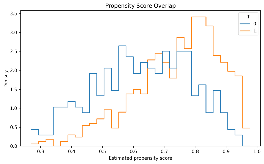
The two curves will not be identical, and that is not the point. What we want to know is whether treated and untreated patients occupy broadly the same region of the score. Clear separation would be a warning that some comparisons have little support in the data.
10. Calculate the IPTW weights
For the ATE:
data['IPTW'] = np.where(
data['T'] == 1,
1 / data['PS'],
1 / (1 - data['PS'])
)
print(data['IPTW'].describe())With our seed (values rounded to three decimals):
count 1000.000
mean 2.004
std 1.565
min 1.025
25% 1.227
50% 1.459
75% 2.076
max 19.429Most weights are modest. The maximum is about 19.43.
This is why the mean weight alone tells you very little: the problem sits in a thin upper tail. A histogram makes it visible.
plt.figure(figsize=(8, 5))
sns.histplot(data['IPTW'], bins=40)
plt.xlabel('IPTW weight')
plt.ylabel('Count')
plt.title('Distribution of IPTW Weights')
plt.tight_layout()
plt.show()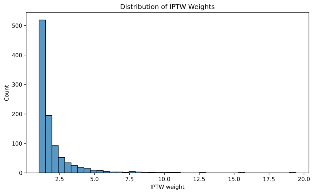
11. A note about stabilized weights
What we have computed are unstabilized ATE weights. A common alternative is to stabilize them.
For treated patients:
and for controls:
The marginal probability in the numerator shrinks the variability of the weights without changing the estimand (under the usual assumptions). Stabilized weights have a mean close to 1, so the weighted sample size stays close to the actual one.
p_treated = data['T'].mean()
data['SW'] = np.where(
data['T'] == 1,
p_treated / data['PS'],
(1 - p_treated) / (1 - data['PS'])
)Here the stabilized weights have mean 1.001 and a maximum of 5.6.
Stabilization and truncation are different operations, though. A stabilized weight can still be extreme if its denominator is tiny. To keep things simple, the rest of the tutorial uses the original unstabilized weights.
12. Apply weight truncation
We truncate at the 1st and 99th percentiles. First the thresholds:
lower = np.quantile(data['IPTW'], 0.01)
upper = np.quantile(data['IPTW'], 0.99)
print(f"1st percentile: {lower:.3f}")
print(f"99th percentile: {upper:.3f}")1st percentile: 1.053
99th percentile: 8.867(With ATE weights, which can never fall below 1, the lower bound does almost nothing. The upper one does the real work.)
Apply the limits:
data['IPTW_trunc'] = np.clip(data['IPTW'], lower, upper)
print(data['IPTW_trunc'].describe())count 1000.000
mean 1.974
std 1.363
min 1.053
25% 1.227
50% 1.459
75% 2.076
max 8.867The maximum drops from 19.429 to 8.867, and the standard deviation of the weights falls from 1.565 to 1.363. That was the aim: no single patient can pull the analysis around quite as much.
Does that make the truncated analysis better? Not by itself. First we have to check whether weighting has done its main job:
Are the baseline covariates now balanced between treatment groups?
13. Assess covariate balance
The most widely used balance measure is the standardized mean difference (SMD). For a continuous variable, a simple version is
Unlike a p-value, the SMD does not grow or shrink with sample size. It answers the question we actually care about: how different are the groups on this variable?
After weighting, we plug in weighted means and weighted variances. For binary variables coded 0/1 the mean is the proportion, so the same code works.
One methodological detail. Some authors and software (the R package cobalt, for instance) keep the unweighted pooled standard deviation in the denominator after weighting, so that before and after values share the same scale. The function below uses weighted variances. Both conventions are defensible; just say which one you used.
13.1 Python function for SMD
def standardized_mean_diff(data, treatment_col, covariate, weights=None):
treated = data[data[treatment_col] == 1]
control = data[data[treatment_col] == 0]
if weights is not None:
w_t = weights.loc[treated.index]
w_c = weights.loc[control.index]
mean_t = np.average(treated[covariate], weights=w_t)
mean_c = np.average(control[covariate], weights=w_c)
var_t = np.average((treated[covariate] - mean_t) ** 2, weights=w_t)
var_c = np.average((control[covariate] - mean_c) ** 2, weights=w_c)
else:
mean_t = treated[covariate].mean()
mean_c = control[covariate].mean()
var_t = treated[covariate].var(ddof=1)
var_c = control[covariate].var(ddof=1)
pooled_std = np.sqrt((var_t + var_c) / 2)
if pooled_std == 0:
return 0
return (mean_t - mean_c) / pooled_stdBefore and after weighting:
smd_before = {
cov: standardized_mean_diff(data, 'T', cov)
for cov in covariates
}
smd_after = {
cov: standardized_mean_diff(data, 'T', cov, weights=data['IPTW_trunc'])
for cov in covariates
}Output:
SMD before weighting:
age 0.192
sex 0.204
comorbidities 0.501
baseline_score 0.508
SMD after truncated IPTW:
age 0.016
sex -0.036
comorbidities 0.063
baseline_score 0.028The sign gives the direction of the difference. For balance we usually look at the absolute SMD:
Before After
age 0.192 0.016
sex 0.204 0.036
comorbidities 0.501 0.063
baseline_score 0.508 0.028A common rule of thumb treats
as acceptable balance. All four variables fall below it after weighting.
Encouraging, yes. But 0.10 is a convention, not a line that separates valid from invalid analyses. And equal means do not imply equal distributions. In a real study it is worth looking at:
- SMDs;
- the full distributions of continuous variables;
- variance ratios;
- clinically important interactions;
- nonlinear transformations of key continuous covariates.
14. Create a Love plot
A Love plot shows balance at a glance.
smd_df = pd.DataFrame({
'Covariate': covariates * 2,
'SMD': (
[abs(v) for v in smd_before.values()]
+ [abs(v) for v in smd_after.values()]
),
'Stage': (
['Before weighting'] * len(covariates)
+ ['After truncated IPTW'] * len(covariates)
)
})
plt.figure(figsize=(8, 5))
sns.scatterplot(
data=smd_df,
x='SMD',
y='Covariate',
hue='Stage',
s=100
)
plt.axvline(x=0.1, linestyle=':', color='grey', label='0.10 threshold')
plt.legend() # redraw the legend so the threshold line is included
plt.xlabel('Absolute standardized mean difference')
plt.title('Covariate Balance Before and After IPTW')
plt.tight_layout()
plt.show()(The explicit plt.legend() call matters: seaborn builds its legend before the vertical line exists, so without it the threshold label never appears.)
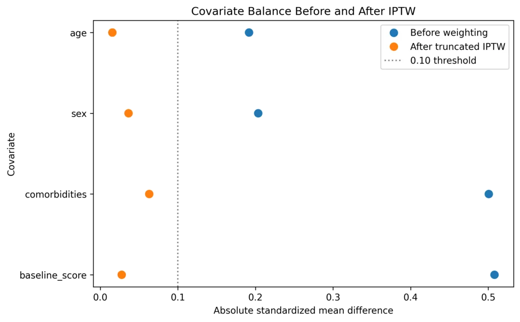
You should see the baseline imbalances collapse toward zero.
The lesson is plain: check balance after building the weights, every time. A propensity-score model can look sophisticated and still leave clinically relevant covariates unbalanced. If it does, it has failed at the only thing it was for.
15. Estimate the treatment effect: the naive analysis
Start with the unadjusted comparison:
unadj_model = smf.ols('Y ~ T', data=data).fit(cov_type='HC1')Treatment coefficient:
T = 3.445 (95% CI 2.954 to 3.935)The true effect used to generate the data was 2.0. The naive analysis overestimates it by more than 70%.
The reason is not mysterious. Treated patients also had the characteristics that raise the outcome. Treatment and baseline prognosis were confounded, and a crude comparison cannot separate them.
16. IPTW-weighted outcome model
Now the weighted model with the truncated weights:
X = sm.add_constant(data[['T']])
y = data['Y']
w = data['IPTW_trunc']
weighted_model = sm.WLS(y, X, weights=w).fit(cov_type='HC1')T = 2.176 (95% CI 1.623 to 2.729)For comparison, it is worth fitting the same model with the untruncated weights as well:
weighted_model_full = sm.WLS(
y, X, weights=data['IPTW']
).fit(cov_type='HC1')T = 2.001 (95% CI 1.363 to 2.639)Side by side:
True effect 2.000
Naive estimate 3.445 (2.954 to 3.935)
Untruncated IPTW estimate 2.001 (1.363 to 2.639)
Truncated IPTW (1st/99th) 2.176 (1.623 to 2.729)Both IPTW estimates are far closer to the truth than the naive one. But the ordering between them is instructive, and not what many readers expect. In this simulation the untruncated estimator is practically unbiased; truncation narrows the confidence interval (width 1.11 instead of 1.28) and, in exchange, shifts the point estimate about 0.18 units away from the true value. That is the bias–variance trade-off from Section 6, made concrete. Here the extreme weights were not noise to be removed. They were carrying information the estimator needed.
It would be wrong to generalize from one simulated dataset in either direction, of course. And the simulation is deliberately kind to IPTW:
- all important confounders are observed;
- the treatment model has the correct functional form;
- there is no meaningful measurement error;
- the treatment effect is constant;
- the outcome-generating mechanism is known.
Clinical datasets are rarely this cooperative.
17. What about standard errors?
Uncertainty needs its own attention in weighted analyses. A frequent mistake is to take the default model-based standard error of a weighted regression and treat it as valid for causal inference. It usually is not.
In this example we used
.fit(cov_type='HC1')which requests a heteroskedasticity-robust sandwich estimator. For a tutorial this is a reasonable choice, and better than reporting the default WLS standard error.
Real IPTW analyses have one more complication, however:
the propensity scores, and therefore the weights, were themselves estimated from the same data.
Our outcome regression treats the weights as fixed and known. They are not. Depending on the estimand, the outcome type, the weighting scheme and the analysis model, a more specialized variance estimator or a bootstrap that re-estimates the propensity model in each resample may be needed. (For ATE weights the robust sandwich that ignores estimation of the propensity score tends to be conservative, but I would not lean on that as a general rule.)
In an applied study, variance estimation belongs in the statistical analysis plan, not in a last-minute fix.
18. What if balance is still poor?
Suppose one or more covariates still show large SMDs after weighting. That is not a reason to abandon IPTW. It is a reason to revisit the propensity-score model, for example with:
- nonlinear terms or splines;
- interaction terms;
- alternative specifications;
- machine-learning methods.
Keep one principle in mind:
The best propensity-score model is not necessarily the one that predicts treatment best.
Its purpose is adequate balance for the chosen estimand. A model with an excellent c-statistic can, if anything, make things worse, by pushing scores toward 0 and 1 and inflating the weights. Model choice should rest on balance diagnostics and subject-matter knowledge rather than on classification accuracy.
19. Sensitivity analysis for truncation
The 1st/99th percentile threshold is a choice, not a standard. Other thresholds are defensible, and it costs very little to try them:
def ess(w):
"""Kish effective sample size."""
return w.sum() ** 2 / (w ** 2).sum()
thresholds = [
(0.0, 1.0), # no truncation
(0.01, 0.99),
(0.025, 0.975),
(0.05, 0.95)
]
for lo, hi in thresholds:
w_tr = np.clip(
data['IPTW'],
np.quantile(data['IPTW'], lo),
np.quantile(data['IPTW'], hi)
)
fit = sm.WLS(y, X, weights=w_tr).fit(cov_type='HC1')
ci_low, ci_high = fit.conf_int().loc['T']
max_smd = max(
abs(standardized_mean_diff(data, 'T', c, weights=w_tr))
for c in covariates
)
print(
f"{lo:>5.3f}-{hi:<5.3f} max w = {w_tr.max():5.2f} "
f"ESS = {ess(w_tr):4.0f} ATE = {fit.params['T']:.3f} "
f"({ci_low:.3f} to {ci_high:.3f}) max |SMD| = {max_smd:.3f}"
)Results with our seed:
Truncation Max w ESS ATE (95% CI) Max |SMD|
none 19.43 621 2.001 (1.363 to 2.639) 0.051
1st/99th 8.87 677 2.176 (1.623 to 2.729) 0.063
2.5th/97.5th 6.42 729 2.324 (1.797 to 2.850) 0.110
5th/95th 4.67 785 2.491 (1.981 to 3.001) 0.173The pattern is hard to miss. As the cap tightens, the effective sample size rises and the intervals narrow. At the same time balance deteriorates (at 2.5% the largest SMD has already crossed 0.10) and the estimate drifts back toward the confounded naive value. Truncation buys precision partly by reintroducing the confounding that the weights were meant to remove.
When a result moves this much between 1% and 5% truncation, the instability is itself a finding, clinically and statistically. Report it.
For each specification it is therefore useful to report:
- the maximum weight;
- the effective sample size;
- covariate balance;
- the treatment-effect estimate with its confidence interval.
Ideally the thresholds are prespecified. Picking the one that gives the most attractive result is, to put it mildly, not a sensitivity analysis.
20. Weight truncation does not solve every problem
Truncation limits the influence of extreme observations. It cannot repair a comparison the data do not support.
If patients with certain characteristics almost never receive treatment, capping their weights creates no new information about what treatment would have done for them. It only hides the gap.
A numerical problem with large weights is often the visible sign of a deeper problem with overlap or positivity.
So look at the propensity-score distributions first, and treat truncation as an analytical decision to be justified rather than a preprocessing step.
21. Other outcomes
Our outcome is continuous, which makes weighted least squares a natural demonstration. For other outcomes the analysis model has to match both the outcome type and the effect measure you are after.
Binary outcomes
Weighted binomial models can be used. Possible estimands include:
- the marginal risk difference;
- the marginal risk ratio;
- the marginal odds ratio.
They are not interchangeable. Decide on the effect measure before choosing the model.
Time-to-event outcomes
Survival outcomes need more care. Weighted Cox models are widely used; a Cox model fitted with IPTW and treatment as the only covariate estimates a marginal hazard ratio, which is not the same quantity as the conditional hazard ratio from a covariate-adjusted model. Variance estimation deserves particular attention here (see Austin, 2016, below).
In Python, lifelines supports weighted Cox regression with robust standard errors. As with any package, check what the estimator actually assumes before using it for a real analysis.
22. The assumptions behind a causal interpretation
Weighting alone does not produce causal inference. A causal reading of an IPTW estimate typically rests on the following.
Exchangeability
Given the measured baseline covariates, there is no important residual confounding. In practice: the important confounders were measured and properly represented in the propensity-score model.
Positivity
Patients with each relevant combination of baseline characteristics have a non-zero probability of receiving every treatment being compared.
Consistency
The treatment a patient actually received corresponds to a well-defined version of the intervention we want to study. This is usually stated together with the absence of interference between patients (one patient’s treatment does not affect another’s outcome), the two forming what is often called SUTVA.
Correct model specification
Strictly speaking this is a modeling requirement rather than an identification assumption, but in practice it matters just as much: the propensity-score and outcome models must be adequate for the job.
None of these can be proven from the data alone. That is why subject-matter knowledge, the kind that knows why a surgeon chose one operation over another, stays essential even in technically sophisticated causal analyses.
23. Complete reproducible Python script
The full example in one block, including the untruncated comparison and the truncation sensitivity analysis.
import numpy as np
import pandas as pd
import statsmodels.api as sm
import statsmodels.formula.api as smf
import matplotlib.pyplot as plt
import seaborn as sns
# ============================================================
# 1. SIMULATE DATA
# ============================================================
np.random.seed(42)
n = 1000
age = np.random.normal(60, 10, n)
sex = np.random.binomial(1, 0.5, n) # 0 = female, 1 = male
comorbidities = np.random.poisson(2, n)
baseline_score = np.random.normal(0, 1, n) # higher = greater risk
# Treatment assignment
logit_p = (
    -1.0
    + 0.02 * age
    + 0.4 * sex
    + 0.3 * comorbidities
    + 0.5 * baseline_score
)
p = 1 / (1 + np.exp(-logit_p))
T = np.random.binomial(1, p, n)
# Outcome (true treatment effect = 2.0)
Y = (
    50
    + 2.0 * T
    + 0.1 * age
    + 0.5 * sex
    + 0.8 * comorbidities
    + 1.0 * baseline_score
    + np.random.normal(0, 3, n)
)
data = pd.DataFrame({
'age': age,
'sex': sex,
'comorbidities': comorbidities,
'baseline_score': baseline_score,
'T': T,
'Y': Y
})
print("\nTreatment groups:")
print(data['T'].value_counts())
covariates = ['age', 'sex', 'comorbidities', 'baseline_score']
# ============================================================
# 2. PROPENSITY SCORE
# ============================================================
formula = 'T ~ ' + ' + '.join(covariates)
ps_model = smf.logit(formula, data=data).fit(disp=False)
data['PS'] = ps_model.predict(data)
print("\nFirst propensity scores:")
print(data[['T', 'PS']].head().round(3))
# ============================================================
# 3. PROPENSITY-SCORE OVERLAP
# ============================================================
plt.figure(figsize=(8, 5))
sns.histplot(
    data=data,
    x='PS',
    hue='T',
    bins=30,
    stat='density',
    common_norm=False,
    element='step',
    fill=False
)
plt.xlabel('Estimated propensity score')
plt.ylabel('Density')
plt.title('Propensity Score Overlap')
plt.tight_layout()
plt.show()
# ============================================================
# 4. IPTW (ATE, unstabilized)
# ============================================================
data['IPTW'] = np.where(
data['T'] == 1,
1 / data['PS'],
1 / (1 - data['PS'])
)
print("\nOriginal IPTW weights:")
print(data['IPTW'].describe())
# ============================================================
# 5. WEIGHT DISTRIBUTION
# ============================================================
plt.figure(figsize=(8, 5))
sns.histplot(data['IPTW'], bins=40)
plt.xlabel('IPTW weight')
plt.ylabel('Count')
plt.title('Distribution of IPTW Weights')
plt.tight_layout()
plt.show()
# ============================================================
# 6. OPTIONAL: STABILIZED WEIGHTS
# ============================================================
p_treated = data['T'].mean()
data['SW'] = np.where(
    data['T'] == 1,
    p_treated / data['PS'],
    (1 - p_treated) / (1 - data['PS'])
)
print("\nStabilized weights:")
print(data['SW'].describe())
# ============================================================
# 7. WEIGHT TRUNCATION (1st / 99th percentile)
# ============================================================
lower = np.quantile(data['IPTW'], 0.01)
upper = np.quantile(data['IPTW'], 0.99)
print(f"\n1st percentile: {lower:.3f}")
print(f"99th percentile: {upper:.3f}")
data['IPTW_trunc'] = np.clip(data['IPTW'], lower, upper)
print("\nTruncated IPTW weights:")
print(data['IPTW_trunc'].describe())
# ============================================================
# 8. STANDARDIZED MEAN DIFFERENCES
# ============================================================
def standardized_mean_diff(data, treatment_col, covariate, weights=None):
    treated = data[data[treatment_col] == 1]
    control = data[data[treatment_col] == 0]
    if weights is not None:
        w_t = weights.loc[treated.index]
        w_c = weights.loc[control.index]
        mean_t = np.average(treated[covariate], weights=w_t)
        mean_c = np.average(control[covariate], weights=w_c)
        var_t = np.average((treated[covariate] - mean_t) ** 2, weights=w_t)
        var_c = np.average((control[covariate] - mean_c) ** 2, weights=w_c)
    else:
        mean_t = treated[covariate].mean()
        mean_c = control[covariate].mean()
        var_t = treated[covariate].var(ddof=1)
        var_c = control[covariate].var(ddof=1)
    pooled_std = np.sqrt((var_t + var_c) / 2)
    if pooled_std == 0:
        return 0
    return (mean_t - mean_c) / pooled_std
smd_before = {
    cov: standardized_mean_diff(data, 'T', cov)
    for cov in covariates
}
smd_after = {
    cov: standardized_mean_diff(data, 'T', cov, weights=data['IPTW_trunc'])
    for cov in covariates
}
print("\nSMD before weighting:")
for cov, value in smd_before.items():
print(f"{cov:20s}: {value:.3f}")
print("\nSMD after truncated IPTW:")
for cov, value in smd_after.items():
print(f"{cov:20s}: {value:.3f}")
# ============================================================
# 9. LOVE PLOT
# ============================================================
smd_df = pd.DataFrame({
'Covariate': covariates * 2,
'SMD': (
[abs(v) for v in smd_before.values()]
+ [abs(v) for v in smd_after.values()]
),
'Stage': (
['Before weighting'] * len(covariates)
+ ['After truncated IPTW'] * len(covariates)
)
})
plt.figure(figsize=(8, 5))
sns.scatterplot(
data=smd_df,
x='SMD',
y='Covariate',
hue='Stage',
s=100
)
plt.axvline(x=0.1, linestyle=':', color='grey', label='0.10 threshold')
plt.legend()
plt.xlabel('Absolute standardized mean difference')
plt.title('Covariate Balance Before and After IPTW')
plt.tight_layout()
plt.show()
# ============================================================
# 10. NAIVE OUTCOME MODEL
# ============================================================
unadj_model = smf.ols('Y ~ T', data=data).fit(cov_type='HC1')
print("\nUnadjusted model:")
print(unadj_model.summary())
# ============================================================
# 11. IPTW-WEIGHTED OUTCOME MODELS
# ============================================================
X = sm.add_constant(data[['T']])
y = data['Y']
weighted_model = sm.WLS(y, X, weights=data['IPTW_trunc']).fit(cov_type='HC1')
print("\nTruncated IPTW model:")
print(weighted_model.summary())
weighted_model_full = sm.WLS(y, X, weights=data['IPTW']).fit(cov_type='HC1')
print("\nUntruncated IPTW model:")
print(weighted_model_full.summary())
# ============================================================
# 12. SENSITIVITY ANALYSIS FOR TRUNCATION
# ============================================================
def ess(w):
"""Kish effective sample size."""
return w.sum() ** 2 / (w ** 2).sum()
thresholds = [(0.0, 1.0), (0.01, 0.99), (0.025, 0.975), (0.05, 0.95)]
print("\nTruncation sensitivity analysis:")
for lo, hi in thresholds:
w_tr = np.clip(
data['IPTW'],
np.quantile(data['IPTW'], lo),
np.quantile(data['IPTW'], hi)
)
fit = sm.WLS(y, X, weights=w_tr).fit(cov_type='HC1')
ci_low, ci_high = fit.conf_int().loc['T']
max_smd = max(
abs(standardized_mean_diff(data, 'T', c, weights=w_tr))
for c in covariates
)
print(
f"{lo:>5.3f}-{hi:<5.3f} max w = {w_tr.max():5.2f} "
f"ESS = {ess(w_tr):4.0f} ATE = {fit.params['T']:.3f} "
f"({ci_low:.3f} to {ci_high:.3f}) max |SMD| = {max_smd:.3f}"
)24. Key lessons
IPTW is conceptually elegant, but a reliable analysis takes much more than simply calculating inverse-probability weights.
A practical workflow:
- Define the causal question and the target estimand.
- Select clinically relevant baseline confounders.
- Estimate the propensity scores.
- Examine propensity-score overlap.
- Calculate the weights.
- Inspect the weight distribution.
- Look at extreme weights and what they say about positivity.
- Truncate only when justified, and report the threshold.
- Check covariate balance after weighting.
- Estimate the treatment effect with an appropriate outcome model.
- Use an appropriate variance estimator.
- Run sensitivity analyses, including the untruncated estimate.
If one idea is worth keeping, it is probably this one:
Propensity-score weighting does not succeed because the propensity model predicts treatment well. It succeeds when it produces a credible comparison between treatment groups for the causal question we want to answer.
Extreme weights are not simply values to get rid of. They are diagnostic information. Sometimes truncation makes an estimator usefully more stable. Sometimes, as in our own example, it quietly trades a small bias for a narrower interval. And sometimes extreme weights are telling us that the data lack the overlap needed for the comparison we are attempting.
Telling these situations apart is most of what using IPTW responsibly means.
Further reading
Austin PC, Stuart EA. Moving towards best practice when using inverse probability of treatment weighting (IPTW) using the propensity score to estimate causal treatment effects in observational studies. Statistics in Medicine. 2015;34:3661–3679. doi:10.1002/sim.6607.
Cole SR, Hernán MA. Constructing inverse probability weights for marginal structural models. American Journal of Epidemiology. 2008;168:656–664. doi:10.1093/aje/kwn164.
Austin PC. Variance estimation when using inverse probability of treatment weighting (IPTW) with survival analysis. Statistics in Medicine. 2016;35:5642–5655. doi:10.1002/sim.7084.