
Introduction: Understanding Calibration Challenges
Consider a thermometer that perfectly identifies when one temperature is higher or lower than another, but consistently reads 5 degrees too high. This thermometer has good discrimination (it correctly ranks temperatures), but poor calibration (its absolute values are inaccurate).
The same problem occurs with clinical risk models such as EuroSCORE: they can be excellent at distinguishing high-risk patients from low-risk ones, but the specific probabilities they provide might not accurately reflect the reality in your population.
Understanding Calibration
The calibration of a predictive model measures how accurately the predicted probabilities match the actual frequency of observed events.
In practical terms:
For optimal calibration, when a model predicts a 20% risk for a group of patients, exactly 20% of those patients should experience the event.
The model overestimates the risk when the event occurs in only 15% of cases.
Conversely, risk is underestimated when the event occurs in 25% of cases.
Why is Calibration Important?
Poor calibration can lead to significant clinical consequences when risk prediction models fail to accurately reflect real-world outcomes. These discrepancies between predicted and actual risk can substantially impact patient care decisions:
Overestimation of risk → Unnecessarily aggressive treatments and interventions that patients don’t need, potentially exposing them to adverse effects, complications, and increased healthcare costs without proportional clinical benefit
Underestimation of risk → Failure to provide appropriate treatments and inadequate attention to truly high-risk patients, potentially resulting in missed opportunities for preventive interventions, delayed recognition of deterioration, and suboptimal management strategies
Calibration Assessment Methods
Graphical methods
Calibration Plot
The most intuitive method to visualize calibration:
Patients are grouped according to their predicted risk levels (0-10%, 10-20%, etc.)
The actual proportion of events is calculated for each group
A graph displays predicted risk (X-axis) against observed risk (Y-axis)
Perfect calibration: all points align with the diagonal line
Points below the line: risk overestimation
Points above the line: risk underestimation

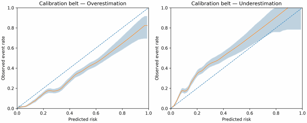
Calibration Belt
An enhanced version of the calibration plot that incorporates confidence bands, helping clinicians distinguish between statistically significant deviations and random variations in the data.
Classic Quantitative Methods
Calibration In The Large (CITL)
This represents the simplest calibration assessment method:
Compares the sum of all predicted events versus observed events
Ratio = Observed events / Predicted events
Value of 1: perfect calibration
Value < 1: global overestimationValue > 1: global underestimation
Hosmer-Lemeshow Test
The classic statistical test for calibration assessment, but use with caution as it has several important limitations:
Divides patients into predetermined risk groups (usually 10 equal-sized groups or deciles of risk)
Systematically compares predicted versus observed event rates within each of these risk groups
Produces a chi-square statistic with a corresponding P-value where values > 0.05 traditionally suggest acceptable calibration (failure to reject the null hypothesis of good fit)
Despite its widespread use in the literature, it has several critical limitations that significantly reduce its utility in modern predictive modeling:
Results depend arbitrarily on the number of groups chosen by the researcher, with different grouping strategies potentially yielding contradictory conclusions from the same dataset
Demonstrates inadequate sensitivity when applied to smaller sample sizes, potentially failing to detect meaningful calibration issues
Paradoxically becomes overly sensitive with very large samples, where clinically insignificant deviations may be flagged as statistically significant problems
Provides only a global assessment without indicating specific regions of the risk spectrum where calibration problems are most pronounced
Produces notably unstable results across different underlying risk distributions, limiting comparability between populations
Advanced Quantitative Methods
Integrated Calibration Index (ICI)
Measures the area between the observed calibration curve and the ideal one:
Values close to 0 indicate excellent calibration
Typically, an ICI < 0.01 is considered good
Provides a comprehensive global measure of calibration error
E50 and E90 (Error Percentiles)
E50 (median absolute error)**:
50% of patients have calibration errors lower than this value, providing a robust central tendency measure that is not influenced by extreme outliers
Indicates the “typical” quality of calibration in your patient population and serves as a reliable benchmark for routine clinical application
E90 (90th percentile of absolute error)**:
Only 10% of patients have calibration errors exceeding this threshold, making it a valuable indicator of the model’s worst-case performance
Indicates how severe the errors can be in the worst cases, which is particularly important when making high-stakes clinical decisions where safety margins are critical
Brier Score
Measures the average “distance” between predictions and actual outcomes:
Formula: Average of (Prediction – Reality)²
Range: 0 (perfect calibration) to 0.25 (random prediction)
Provides a comprehensive measure that combines both calibration and discrimination
Alternative Statistical Tests
Spiegelhalter’s Z-test
Provides a comprehensive single Z-score for overall calibration assessment, making it easier to interpret compared to multiple metrics
Statistical interpretation follows standard normal distribution where |Z| < 1.96 indicates acceptable calibration at the 95% confidence level
More robust than Hosmer-Lemeshow for large samples, as it doesn’t suffer from the same sensitivity issues when sample sizes increase
Particularly useful for comparing calibration across different predictive models applied to the same population
Maintains consistent performance regardless of the underlying risk distribution in your patient cohort
Le Cessie-Van Houwelingen Test
Does not require arbitrary division into groups, making it more consistent and reliable than methods that depend on subjective grouping choices
Particularly suitable for logistic regression models and provides a more sophisticated assessment of the goodness-of-fit for probability predictions in clinical settings
Less influenced by data distribution anomalies, offering more robust performance across diverse patient populations with varying risk profiles
Evaluates the overall calibration quality by examining the squared differences between observed outcomes and predicted probabilities
Maintains statistical power even with smaller sample sizes, making it valuable for specialized clinical applications with limited available data
Summary Table: Calibration Assessment Methods
| Method | Type | Interpretation | Advantages | Limitations |
| Calibration Plot | Graph | Points on diagonal = perfect | Visual, intuitive | Subjective, depends on grouping |
| Calibration Belt | Graph | Diagonal + confidence bands | Shows statistical significance | More complex interpretation |
| CITL | Numeric | 1 = perfect, <1 = overestimation, >1 = underestimation | Simple single value | Only overall assessment |
| Hosmer-Lemeshow test | Test | p>0.05 = accettable calibration | Classic, widely known | Unstable, poorly informative |
| ICI | Numeric | 0 = perfect, <0.01 = good | Robust global measure | Doesn’t pinpoint issues |
| E50/E90 | Numeric | Median/90th percentile of errors | Clinically interpretable | E90 sensitive to outliers |
| Brier Score | Numeric | 0 = perfect, <0.25 = useful | Comprehensive measure | Combines multiple aspects |
| Spiegelhalter Z-test | Test | |Z| < 1.96 = acceptable | Single standardized score | Less intuitive clinically |
| Le Cessie test | Test | p > 0.05 = acceptable | No arbitrary grouping | More complex than H-L |
Correcting Calibration Errors
Platt Scaling
Platt Scaling represents the most extensively adopted and widely implemented methodology for correcting calibration issues in predictive models across various clinical domains:
How it works:
Applies a specialized form of logistic regression transformation directly to the original prediction outputs, effectively recalibrating them without altering their fundamental ranking properties
Formula: P_calibrated = 1 / (1 + exp(A × original_score + B)), where the equation creates a sigmoid-shaped adjustment that can correct both over-prediction and under-prediction issues across the risk spectrum
Parameters A and B are statistically derived using your local patient population data through maximum likelihood estimation, ensuring the calibration correction is specifically tailored to your clinical context
Advantages:
Simple to implement in most statistical packages and clinical decision support systems without requiring complex computational resources
Maintains the critical rank-order of predictions, ensuring the discrimination ability of the model (its capacity to separate high-risk from low-risk patients) remains completely unchanged
Effective for addressing most common calibration biases encountered in clinical predictive models, including systematic over-prediction and under-prediction patterns
Disadvantages:
Requires a separate, independent dataset for calibration parameter estimation and subsequent validation to avoid overfitting, which may be challenging in resource-limited settings
Assumes a sigmoidal relationship between the original scores and observed outcomes, which may not adequately correct more complex non-monotonic calibration issues that occasionally arise in heterogeneous patient populations
Temperature Scaling
Temperature Scaling represents a streamlined and computationally efficient variant of the more complex Platt Scaling methodology, providing a more accessible approach to model recalibration while maintaining essential corrective capabilities:
Employs a single correction parameter (temperature) that functions as a scaling factor applied uniformly across all predictions, significantly reducing computational complexity while still addressing systematic calibration issues
Offers enhanced implementation simplicity and reduced computational requirements, making it particularly suitable for resource-constrained clinical environments, though it provides less flexibility for correcting complex non-linear calibration patterns compared to multi-parameter approaches
Isotonic Regression
Does not assume a specific form of the relationship between predicted probabilities and actual outcomes, allowing for more flexible correction of complex calibration errors across different risk ranges
Particularly useful when the bias is very irregular or non-monotonic, such as when a model simultaneously overestimates risk in some patients while underestimating it in others, depending on where they fall in the risk spectrum
More complex to implement than simpler methods like Platt scaling, requiring specialized algorithms and additional computational resources, though the improved calibration accuracy often justifies this increased complexity in high-stakes clinical applications
Practical Advice
Begin calibration analysis with “raw” data to evaluate a model’s actual clinical performance in your specific patient population. This initial assessment often provides sufficient insight into the model’s direct applicability to your clinical practice.
If needed, proceed with calibration. This process isolates the model’s intrinsic predictive ability and enables fairer comparisons between models developed across different populations.
Follow this sequence: conduct raw data analysis first, then calibrate if necessary, and finally evaluate post-calibration performance.
You can validate calibration using several approaches:
Temporal split: Use historical data for calibration and recent data for validation
Cross-validation: Divide your dataset into multiple parts for more robust validation
Geographic split: Calibrate using data from one center and validate with data from others
Goal-oriented approach
For Daily Clinical Use
Incorporate calibration plots alongside ICI and E50/E90 metrics as your primary assessment tools to efficiently evaluate model performance in routine clinical practice
These methodologies provide an optimal balance between statistical rigor and intuitive interpretation, allowing healthcare providers to quickly grasp calibration quality without requiring extensive statistical expertise
The visual nature of calibration plots coupled with the numerical precision of ICI and E50/E90 metrics creates a comprehensive assessment framework that can be readily communicated to clinical teams during decision-making processes
For Scientific Research
Implement a multi-dimensional approach by strategically combining complementary graphical representations and quantitative metrics to capture the full spectrum of calibration characteristics
Establish methodological robustness by utilizing multiple independent indicators that collectively provide a comprehensive assessment of model calibration across different dimensions of performance
Exercise caution regarding over-reliance on the Hosmer-Lemeshow test due to its known limitations with large sample sizes and sensitivity to arbitrary grouping decisions
Maintain a dual focus on both statistical significance and clinical relevance by contextualizing calibration findings within the specific medical domain and intended application, recognizing that statistically significant deviations may not always translate to clinically meaningful differences in patient outcomes
For Developing New Models
Integrate calibration assessment into the earliest phases of model development rather than treating it as an afterthought, establishing it as a core design consideration alongside discrimination metrics
Implement rigorous methodological standards by systematically setting aside truly independent validation datasets that remain completely untouched during model development and initial calibration phases
Ensure comprehensive documentation of all calibration methodologies, decision thresholds, and statistical approaches used throughout the development process to enhance transparency and facilitate proper implementation by other researchers and clinicians
Consider the temporal stability of calibration by designing periodic reassessment protocols that can identify calibration drift as patient populations and clinical practices evolve over time
Best Practices
Always use multiple methods – combine graphical, quantitative, and (when appropriate) statistical test approaches
Avoid using Hosmer-Lemeshow test – opt for more robust alternatives
Look beyond statistical significance – prioritize clinical relevance
Reserve independent data for validation when applying calibration corrections
Document thoroughly all methods used and defined acceptability thresholds
1. ALWAYS start with: Calibration plot + CITL
↓
2. If CITL ≠ 1 → Global calibration problem
↓
3. Add: ICI + E50 + E90 to quantify
↓
4. If statistical test needed: - Small sample (<500): Le Cessie test - Large sample (>500): Spiegelhalter test - NEVER use Hosmer-Lemeshow alone
↓
5. If correction needed: - Simple: Platt Scaling - Complex: Isotonic Regression
↓
6. ALWAYS validate on independent data
References and Suggested Literature
Hosmer-Lemeshow test
Hosmer, D.W., Lemeshow, S. (1980). A goodness-of-fit tests for the multiple logistic regression model. Communications in Statistics, 10, 1043-1069[1]
Kramer, A.A., Zimmerman, J.E. (2007). Assessing the calibration of mortality benchmarks in critical care: The Hosmer-Lemeshow test revisited. Critical Care Medicine, 35(9), 2052-2056[2]
Integrated Calibration Index (ICI)
Austin, P.C., Steyerberg, E.W. (2019). The Integrated Calibration Index (ICI) and related metrics for quantifying the calibration of logistic regression models. Statistics in Medicine, 38(21), 4051-4065[3]
Calibration Plot
Austin, P.C., Steyerberg, E.W. (2014). Graphical assessment of internal and external calibration of logistic regression models by using loess smoothers. Statistics in Medicine, 33(3), 517-535[4]
Calibration Belt
Finazzi, S., Poole, D., Luciani, D., Cogo, P.E., Bertolini, G. (2011). Calibration belt for quality-of-care assessment based on dichotomous outcomes. PLOS ONE, 6(2), e16110[6]
Brier Score
Brier, G.W. (1950). Verification of forecasts expressed in terms of probability. Monthly Weather Review, 78(1), 1-3
Le Cessie-van Houwelingen test
le Cessie, S., van Houwelingen, J.C. (1991). A goodness-of-fit test for binary regression models, based on smoothing methods. Biometrics, 47(4), 1267-1282[5]
Platt Scaling
Platt, J. (1999). Probabilistic outputs for support vector machines and comparisons to regularized likelihood methods. Advances in Large Margin Classifiers, 61-74
Review
Van Calster, B., McLernon, D.J., van Smeden, M., Wynants, L., Steyerberg, E.W. (2019). Calibration: the Achilles heel of predictive analytics. BMC Medicine, 17, 230[7]
Huang, Y., Li, W., Macheret, F., Gabriel, R.A., Ohno-Machado, L. (2020). A tutorial on calibration measurements and calibration models for clinical prediction models. Journal of Biomedical and Health Informatics, 24(4), 1079-1090[8]
Conclusions
Calibration isn’t merely a technical consideration but a fundamental requirement for the safe and effective use of predictive models in medicine. A well-calibrated model accurately identifies not just who faces risk but precisely how much risk they face, enabling clinicians to make more informed and appropriate decisions.