
Mean heart rate is one of the most familiar numbers in medicine. Useful, immediate, and often enough for a first description. Yet every average carries the same defect: it compresses into a single value everything that happened over time. Two patients can share a mean of 70 beats per minute (bpm) and, across the same recording window, behave in entirely different ways.
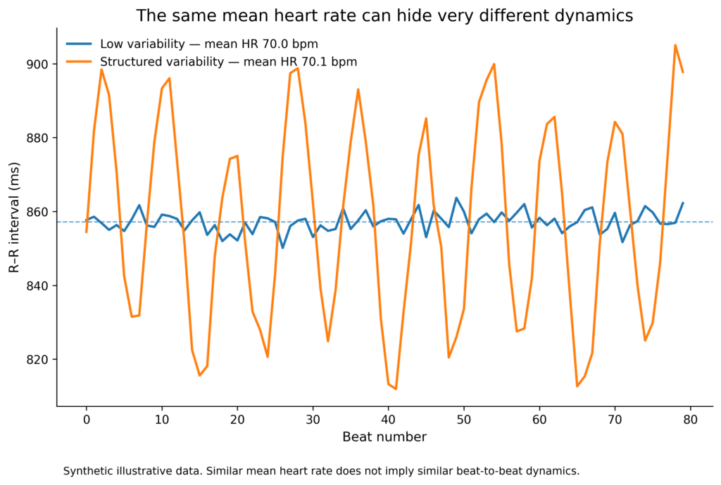
Heart Rate Variability (HRV) was developed to describe precisely that missing part: not how fast the heart is beating, but how the intervals between consecutive beats change from one moment to the next.
What HRV reflects is a compound of sinus node behaviour, autonomic traffic, respiration, baroreflex activity, and a handful of other physiological influences that are difficult to separate cleanly. That compound nature is why HRV became a staple of cardiovascular research and of digital monitoring, and also why interpretative shortcuts around it are so easy to take. No single metric can be labelled “good” or “bad” on its own.
Central idea: mean heart rate describes the level; HRV describes the dynamics. Understanding it requires both physiological intuition and a minimum of mathematics.
1. The same average, two different rhythms
Take two series of R–R intervals, meaning the intervals between consecutive R peaks on the electrocardiogram (ECG), with an almost identical mean heart rate.
| Profile | R–R intervals (ms, milliseconds) | Intuitive interpretation |
|---|---|---|
| A | 857, 857, 857, 857, 857, 857 ms | Almost perfectly regular rhythm |
| B | 820, 890, 835, 880, 845, 875 ms | Greater beat-to-beat variability |
The average erases that difference. HRV tries to recover it.
A caveat worth stating immediately, because it is the source of most misreadings: greater variability is not automatically healthier variability. Premature beats, atrial fibrillation, noise, or a detection algorithm that fires twice on the same complex will all inflate irregularity without any physiology behind it.
2. Signal quality comes before HRV
Everything starts with R-peak detection and the construction of the R–R series. Under ideal conditions the analysis runs on normal-to-normal (NN) intervals, that is, intervals between valid sinus beats, once ectopic beats and artefacts have been excluded or corrected.
A reasonable pipeline includes:
- ECG acquisition and R-peak detection;
- quality control and identification of artefacts or ectopic beats;
- construction of the NN interval series;
- possible interpolation of missing points, using explicitly defined criteria;
- calculation of time-domain metrics;
- possible resampling for spectral analysis;
- calculation of nonlinear metrics;
- interpretation together with respiration, cardiac rhythm, medications, and clinical context.
This is not a minor technical preamble. Anyone who has spent time in front of postoperative telemetry knows how much a shifted electrode, a shivering patient, or a poorly adherent pad can do to a tracing: a handful of wrong intervals is enough to move the standard deviation of NN intervals (SDNN), the root mean square of successive differences (RMSSD), or Sample Entropy well outside their true range. The risk, in other words, is to describe an artefact as though it were a physiological trait.
3. Time domain: how much variability is present?
Time-domain metrics are the simplest entry point. They describe how widely NN intervals are distributed, and how much they shift from one beat to the next.
3.1 SDNN: overall variability
SDNN (standard deviation of NN intervals) is the standard deviation of the NN intervals:
where:
A higher SDNN means greater dispersion of the intervals within the observed window.
Duration, though, changes the meaning of the number. An SDNN computed over five minutes and an SDNN computed over 24 hours are not describing the same phenomenon, and treating them as interchangeable is one of the more common errors in the literature. Over a full day, circadian rhythm, sleep, physical activity, and even ambient temperature all feed into the observed variability.
3.2 RMSSD: beat-to-beat variability
RMSSD (root mean square of successive differences) looks at differences between consecutive intervals:
It is sensitive to rapid variability. In short-term recordings during sinus rhythm, RMSSD is conventionally read as being strongly influenced by vagal modulation, and it has the practical advantage of being relatively robust to recording length.
3.3 pNN50: percentage of successive NN intervals differing by more than 50 ms
The pNN50 is the percentage of consecutive NN interval pairs differing by more than 50 milliseconds (ms):
A historical measure of short-term variability, still reported for continuity with older studies. RMSSD tends to be preferred today because it uses the whole distribution of successive differences instead of collapsing it against a fixed 50 ms threshold, which is arbitrary and behaves poorly at low variability.
4. Frequency domain: which oscillations make up HRV?
The R–R series can also be read as a signal built from slower and faster oscillations. Spectral analysis estimates how much signal “power” falls into different frequency ranges.
Applying the Fast Fourier Transform (FFT), or more commonly estimating power spectral density with Welch’s method, requires transforming the R–R intervals into a uniformly sampled series, typically at 4 hertz (Hz). That resampling step is itself an assumption, and it is rarely discussed in the results section of papers that depend on it.
The power within a band can be understood as the area under the spectral density between two frequencies:
The conventional bands are:
| Band | Frequency (Hz, hertz) | Cautious interpretation |
|---|---|---|
| VLF (very low frequency) | 0.0033–0.04 Hz | Very slow component; poorly reliable in short recordings and not attributable to a single physiological mechanism |
| LF (low frequency) | 0.04–0.15 Hz | Mainly reflects baroreflex-related dynamics and mixed autonomic contributions |
| HF (high frequency) | 0.15–0.40 Hz | Strongly related to respiratory sinus arrhythmia and vagal modulation when respiration falls within this band |

Then there is the low-frequency to high-frequency ratio (LF/HF). For roughly two decades it was presented as an index of “sympathovagal balance”, and the label stuck well beyond the point at which it was defensible. Contrary to that reading, LF is not a proxy for sympathetic activity, and HF does not capture the whole parasympathetic contribution. Reporting the ratio is fine; assigning it a single physiological meaning is not.
Respiration deserves its own line. At roughly 15 breaths per minute, respiratory modulation sits comfortably inside the HF band. Slow breathing, of the kind used in relaxation protocols or seen in a sedated patient, can push it down toward LF, at which point the spectral picture changes without any change in autonomic state. If respiratory frequency is unknown, physiological interpretation of the spectrum becomes considerably more speculative than most published analyses admit.
5. It is not enough to know how much the signal varies: how it varies also matters
Two signals can share mean and variance and still be organised differently. One series may be almost mechanically regular; another may be complex, or simply less predictable. Nonlinear metrics exist to capture that difference.
5.1 Sample Entropy
Sample Entropy (SampEn) measures, in intuitive terms, how likely similar patterns of a given length are to remain similar when extended by one more point.
Its compact form:
where B is the number (or probability) of pairs of similar patterns of length m, and A the pairs that remain similar at length m + 1.
In HRV work the usual choices are:
m = 2
with tolerance r around:
of the signal.
The tempting reading, higher equals better, is wrong. A very low SampEn points to a highly predictable signal; a higher value points to greater irregularity. But noise raises it too, and so do arrhythmias, and so does a shorter series. Or more precisely: SampEn is a property of the processed series, not of the patient, and it inherits every decision made upstream in preprocessing.
5.2 Poincaré plot: transforming the sequence into geometry
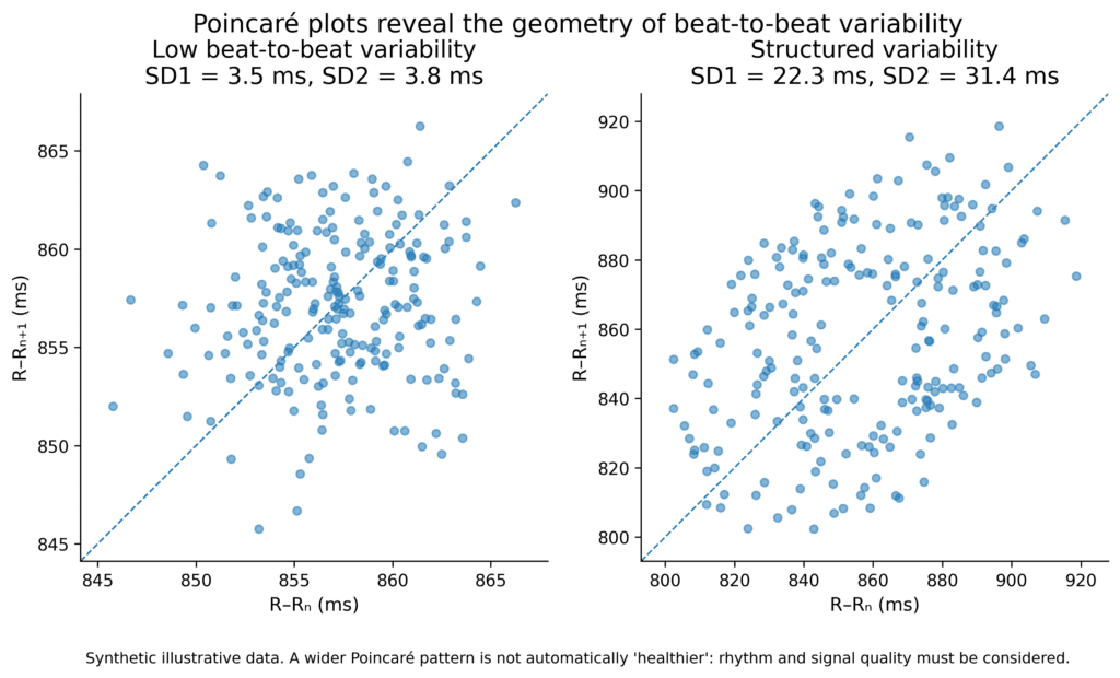
In a Poincaré plot each NN interval goes on the x-axis and the next one on the y-axis. The resulting cloud gives an immediate visual sense of the dynamics, which is why it survives in clinical practice despite being the least mathematically sophisticated tool in this article.
Two descriptors dominate:
- standard deviation 1 (SD1), related to transverse dispersion;
- standard deviation 2 (SD2), related to longitudinal dispersion.
A useful relationship:
SD1 therefore tracks short-term variability, while SD2 describes a slower, more global component. The SD1/SD2 ratio is sometimes reported as a descriptor of the geometry of the cloud, though its incremental value over RMSSD is debatable.
5.3 Detrended Fluctuation Analysis: the fractal component
Detrended Fluctuation Analysis (DFA) asks how fluctuations in the signal correlate across different time scales.
The exponent α₁ describes short-term correlations and has been examined in heart failure, post-infarction populations, and during exercise. As with the other nonlinear metrics, no universal cut-off transfers cleanly across populations and recording conditions, and the values published for one device rarely reproduce on another.
6. Can HRV predict cardiovascular events?
Reduced HRV has been associated with worse prognosis and higher mortality across a long list of studies. The distinction that matters here is between association, predictive ability, and clinical utility, three things that are routinely conflated.
A metric can be statistically associated with an outcome and still fail to improve a predictive model enough to change any decision.
HRV is best treated, then, as a family of signal-derived biomarkers rather than as a test. Its potential value shows up only when these measures add something beyond age, medical history, diabetes, ventricular function, and the medications already on the chart.
7. A predictive model, without turning the article into a regression textbook
For a binary outcome, say a cardiovascular event within three years, logistic regression is the natural starting point.
Its essential structure:
The point is not to pack in as many terms as the software will accept. It is to choose a small number of features with a stated rationale, avoid redundancy (SDNN and RMSSD are correlated, and SD1 is essentially RMSSD rescaled), and check that the added complexity buys real predictive improvement.
Interactions can matter, HRV × age or HRV × diabetes among them, since the same metric may behave differently in different clinical contexts. They should be specified a priori rather than harvested from the data after the fact.
In practice I would compare three levels:
- a baseline clinical model;
- the clinical model plus a small number of conventional HRV metrics;
- the clinical model plus HRV and one or two complexity measures, with clinically justified interactions where appropriate.
Evaluation needs discrimination and calibration, the Brier score, bootstrap or cross-validation for internal validation, and, whenever it can be arranged, genuine external validation. Internal validation alone tends to flatter the model.
One practical note: restricted cubic splines are usually preferable to forcing a straight line between an HRV metric and risk. The relationship is rarely linear, and at the extremes it sometimes reverses.
8. A Python example: from the R–R vector to the main HRV metrics
A little code helps, because it makes concrete what happens between the signal and the final number.
The example below is deliberately didactic. It assumes the intervals have already been cleaned, and it is not a substitute for a clinical preprocessing pipeline.
import numpy as np
from scipy.signal import welch


def sdnn(nn_ms):
    nn = np.asarray(nn_ms, dtype=float)
    return np.std(nn, ddof=1)


def rmssd(nn_ms):
    nn = np.asarray(nn_ms, dtype=float)
    diff = np.diff(nn)
    return np.sqrt(np.mean(diff**2))


def pnn50(nn_ms):
    nn = np.asarray(nn_ms, dtype=float)
    diff = np.abs(np.diff(nn))
    return 100 * np.mean(diff > 50)


def sample_entropy(nn_ms, m=2, r_frac=0.2):
    x = np.asarray(nn_ms, dtype=float)
    r = r_frac * np.std(x, ddof=1)

    def count_matches(length):
        templates = np.array([
            x[i:i+length]
            for i in range(len(x) - length + 1)
        ])

        count = 0

        for i in range(len(templates)):
            for j in range(i + 1, len(templates)):
                if np.max(np.abs(templates[i] - templates[j])) <= r:
                    count += 1

        return count

    B = count_matches(m)
    A = count_matches(m + 1)

    if A == 0 or B == 0:
        return np.nan

    return -np.log(A / B)


def frequency_domain(nn_ms, fs_interp=4.0):
    nn = np.asarray(nn_ms, dtype=float)

    # cumulative time in seconds
    t = np.cumsum(nn) / 1000.0
    t = t - t[0]

    # uniform resampling
    t_uniform = np.arange(0, t[-1], 1 / fs_interp)
    nn_uniform = np.interp(t_uniform, t, nn)
    nn_uniform -= np.mean(nn_uniform)

    f, psd = welch(
        nn_uniform,
        fs=fs_interp,
        nperseg=min(256, len(nn_uniform))
    )

    def band_power(low, high):
        mask = (f >= low) & (f < high)

        if np.sum(mask) < 2:
            return np.nan

        return np.trapezoid(psd[mask], f[mask])

    vlf = band_power(0.0033, 0.04)
    lf = band_power(0.04, 0.15)
    hf = band_power(0.15, 0.40)

    return {
        "VLF": vlf,
        "LF": lf,
        "HF": hf,
        "LF_HF": lf / hf if hf and hf > 0 else np.nan,
}Four ideas come through in these few lines:
- SDNN works on overall dispersion;
- RMSSD compares consecutive beats;
- SampEn compares patterns;
- spectral analysis needs a uniform time axis before it can estimate anything.
A real implementation would need considerably more: checks on minimum recording duration, handling of ectopic beats and artefacts, some assessment of stationarity, a signal-quality index, and explicit choices about spectral-estimation parameters.
The nested loop in sample_entropy is O(N²) and will crawl on 24-hour recordings. For anything beyond a teaching example, use one of the validated and vectorised implementations available in the established HRV libraries.
9. Three patients, the same mean heart rate
This table is the whole argument in miniature: the average is not false, it is incomplete. What is interesting sits in the temporal structure the average necessarily discards.
| Patient | Mean heart rate (HR) | SDNN/RMSSD | SampEn | Possible interpretation |
|---|---|---|---|---|
| A | 70 bpm | Very low | Low | Very regular rhythm; possibly reduced adaptability, but interpretation requires context |
| B | 70 bpm | Moderate | Intermediate | Pattern compatible with physiological variability in a clean sinus-rhythm signal |
| C | 70 bpm | High | Very high | Before calling this “high HRV”, rule out ectopic beats, atrial fibrillation, and artefacts |
Patient C is the one that should give pause. In my experience the reflex to read high variability as good autonomic health is strong, and it is exactly the case where the tracing deserves a second look before the number is trusted.
10. The limitations that really matter
Most of the limitations are methodological rather than physiological:
- artefacts and detection errors can move HRV metrics substantially;
- premature beats and atrial fibrillation generate R–R irregularity that has nothing to do with richer autonomic modulation;
- respiration drives a large share of the HF component and can contaminate LF;
- beta-blockers, antiarrhythmics, anticholinergics, and several other drug classes act on both heart rate and HRV;
- recording duration is not a detail: five-minute and 24-hour measurements are not interchangeable;
- posture, activity, sleep, time of day, and measurement conditions need standardising before subjects or sessions are compared;
- nonlinear metrics look promising but remain poorly standardised, with no universal cut-offs;
- a prognostic association proves neither causality nor clinical usefulness.
Consumer wearables add a further layer, since most estimate inter-beat intervals from photoplethysmography rather than from an ECG. Whether values obtained that way are comparable to ECG-derived HRV is, as far as I can tell, still unsettled across devices and conditions.
11. Final message
HRV is interesting because it forces us to look at the heart as a dynamic system rather than as a rate.
SDNN and RMSSD describe how much the signal varies.
The spectrum shows at which frequencies the oscillations occur.
Sample Entropy, Poincaré analysis, and DFA attempt to describe how that variability is organised.
The future will probably not turn on a single RMSSD or SampEn threshold, but on the integration of several signal characteristics with clinical context.
With wearable devices, continuous monitoring, and predictive models that survive external validation, cardiac time series may become a far richer source of information than mean heart rate alone. That, at least, is the reasonable expectation. Whether it translates into decisions at the bedside is a different question, and one the field has not yet answered.
Heart rate tells us how fast the heart is beating. HRV helps us understand how that rhythm changes over time. It is within this dynamic behavior—not within a single number—that part of the physiological and prognostic information may be found.
Essential bibliography
- Task Force of the European Society of Cardiology and the North American Society of Pacing and Electrophysiology. Heart rate variability: standards of measurement, physiological interpretation and clinical use. European Heart Journal. 1996;17(3):354–381. DOI: 10.1093/oxfordjournals.eurheartj.a014868 · PubMed
- Sassi R, Cerutti S, Lombardi F, Malik M, Huikuri HV, Peng CK, Schmidt G, Yamamoto Y. Advances in heart rate variability signal analysis: joint position statement by the e-Cardiology ESC Working Group and the European Heart Rhythm Association co-endorsed by the Asia Pacific Heart Rhythm Society. Europace. 2015;17(9):1341–1353. DOI: 10.1093/europace/euv015 · PubMed
- Henriques T, Ribeiro M, Teixeira A, Castro L, Antunes L, Costa-Santos C. Nonlinear Methods Most Applied to Heart-Rate Time Series: A Review. Entropy (Basel). 2020;22(3):309. DOI: 10.3390/e22030309 · PubMed
- Faust O, Hong W, Loh HW, Xu S, Tan RS, Chakraborty S, Barua PD, Molinari F, Acharya UR. Heart rate variability for medical decision support systems: A review. Computers in Biology and Medicine. 2022;145:105407. DOI: 10.1016/j.compbiomed.2022.105407 · PubMed
- Jarczok MN, Weimer K, Braun C, Williams DP, Thayer JF, Gündel HO, Balint EM. Heart rate variability in the prediction of mortality: A systematic review and meta-analysis of healthy and patient populations. Neuroscience & Biobehavioral Reviews. 2022;143:104907. DOI: 10.1016/j.neubiorev.2022.104907 · PubMed