Last updated: October 2026
Author: Michele D. Pierri
Reading time: 25–30 minutes
Introduction
A 78-year-old woman sits in front of me with an echocardiogram showing severe aortic stenosis. She has already decided on a biological valve. Her question is the one every surgeon hears:
“How long will it last?”
The honest answer usually comes from a curve. Somewhere in a durability paper there is a figure labelled “freedom from reoperation”, and at ten years it reads, say, 85%. So we say that roughly one patient in seven will need another procedure within a decade.
For her, that sentence is probably wrong. The problem is not the valve or the paper. The curve was built to answer a different question.
Most valve durability curves are Kaplan–Meier curves. Kaplan–Meier handles censoring beautifully, but it has no notion of competing risks, and that blind spot shapes how we talk about valve durability. Death is the obvious one. A patient who dies with a working prosthesis will never be reoperated. If death is treated as ordinary censoring, the method quietly assumes she would have gone on to fail at the same rate as the survivors. In an elderly population, where death is common and early, that assumption turns a hypothetical quantity into a number that looks like her personal risk.
This matters more today than it did ten years ago. Transcatheter valves are moving into younger and lower-risk patients. The 2025 ESC/EACTS guidelines have shifted the age thresholds. Long-term durability data from randomized trials such as PARTNER 3 are now being read line by line by heart teams [1, 2]. If we are going to argue about a few percentage points of valve failure at seven or ten years, we should agree on what those percentages mean.
This post covers:
- what Kaplan–Meier really estimates when patients die;
- what the cumulative incidence function estimates instead, with a worked example you can do by hand;
- the difference between cause-specific and subdistribution (Fine–Gray) hazards, and when to use each;
- a Python simulation in which the same valve is reoperated in one 80-year-old in three according to Kaplan–Meier, and in one in eight in reality, and why both numbers are “correct”;
- a checklist for reading, and writing, valve durability papers.
If you need a refresher on censoring and the Kaplan–Meier estimator, the Survival Analysis page on this site covers the basics.
1. Two questions hidden in one
“What is the probability that this valve will need reoperation within ten years?” sounds like one question. It is actually two.
Question A: a net, device-centred question. Among patients who remain available to experience valve failure, how fast does reoperation for structural valve deterioration occur? A Kaplan–Meier analysis that censors death is closely related to this question. It is often useful when the scientific interest is the valve-failure process itself.
It is tempting to translate this into: “What would happen to the valve if the patient could not die?” That is a useful intuition, but it is a stronger, counterfactual interpretation. The observed data do not literally show us a world in which death has been switched off.
Question B: an observed-world patient question. In the real world, where people may die before their prosthesis fails, what proportion of patients will actually undergo reoperation within ten years? This is the question my 78-year-old patient is usually asking. It is also the question a health system asks when it plans how many redo procedures or valve-in-valve interventions it will need.
There is one more nuance. A raw cumulative-incidence curve is a population estimate: it tells us what happened, on average, in patients like those in the study. To estimate the probability for one particular 78-year-old woman, we need a conditional prediction that uses her characteristics and is well calibrated in a relevant population.
The two population-level answers can differ enormously. The distinction is not new to cardiac surgery. In 2008 the joint AATS/EACTS/STS guidelines for reporting outcomes after valve interventions noted that, because Kaplan–Meier assumes patient immortality, it “overestimates the actual probability of event occurrence”. They recommended the cumulative incidence method whenever valve performance has to be translated into patient risk [3]. The EJCTS/ICVTS statistical guidelines put it more bluntly: ignoring competing risks can lead to biased estimates, and the cumulative incidence function is the standard way to summarize such data [4].
Yet the Kaplan–Meier “freedom from” curve is still the default figure in many durability papers. Why?
Partly habit. Partly because it gives the valve the benefit of the doubt. And partly because many of us were never taught what the curve assumes.
2. What Kaplan–Meier assumes
The Kaplan–Meier estimator [5] multiplies conditional probabilities of “surviving” each event time:
\[
\hat S_{KM}(t) = \prod_{t_j \le t}\left(1 – \frac{d_j}{n_j}\right)
\]
where \(d_j\) is the number of events at time \(t_j\) and \(n_j\) the number of patients still at risk just before it. Censored patients leave the risk set without contributing an event.
The crucial assumption is independent (non-informative) censoring. A censored patient is assumed to have the same future risk as the patients who remain under observation. For administrative censoring, which simply means the study ended, the assumption is usually reasonable: the patient is still alive, still carrying her valve, and would have been observed had the study continued.
Death is different in kind:
- A patient who has died is no longer at risk of reoperation. There is no future in which she is reoperated.
- Treating her as censored means the estimator redistributes her “share” of future reoperations to the survivors, as if she were still out there, waiting to fail.
When you compute \(1 – \hat S_{KM}(t)\) with death censored, you estimate a net failure quantity: the event-of-interest process is followed while deaths are removed from the risk set as censored observations. Surgeons of the 1990s called this the actuarial risk, as opposed to the actual risk [6, 7].
A useful way to remember the difference is:
- ordinary censoring: we do not know what happened next;
- death as a competing event: we know reoperation can no longer happen.
Those are not the same situation.
Two further points are easy to miss.
First, the common phrase “the probability of reoperation if nobody died” is an intuition, not something directly observed. Giving \(1-\hat S_{KM}\) that literal counterfactual meaning requires additional assumptions about the relationship between death and valve failure [8, 21]. The frail patient who dies of heart failure at year four may have had a different underlying valve-failure trajectory from a patient who survives to year ten.
Second, the gap grows with competing mortality. In a 55-year-old undergoing a Ross procedure, death is rare in the first decade and 1 − KM is close to the actual risk. In an 80-year-old receiving a transcatheter valve, the two quantities can differ by a factor of two or three, as we will see.
3. The cumulative incidence function, worked out by hand
The cumulative incidence function (CIF) for event type \(k\) is simply the probability of experiencing event \(k\) first, before any competing event, by time \(t\):
\[
F_k(t) = P(T \le t,\ \text{cause} = k)
\]
Its non-parametric estimator is the Aalen–Johansen estimator [9]:
\[
\hat F_k(t) = \sum_{t_j \le t} \hat S(t_{j-1}) \cdot \frac{d_{kj}}{n_j}
\]
The formula is less intimidating than it looks. \(\hat S(t_{j-1})\) is the Kaplan–Meier probability of being alive and free of any event just before \(t_j\), counting all event types as events. \(d_{kj}/n_j\) is the proportion of those at risk who experience event \(k\) at \(t_j\). So the CIF adds up, over time, “the probability of still being around” times “the probability of the event of interest happening now”. Patients who have died stop contributing, because they are no longer “around”.
A three-year example
Consider 100 patients followed for three years, with no censoring at all, to keep things clean.
| Year | At risk | Reoperations | Deaths | 1 − KM (death censored) | Aalen–Johansen CIF |
|---|---|---|---|---|---|
| 1 | 100 | 5 | 20 | 5.0% | 5.0% |
| 2 | 75 | 6 | 15 | 12.6% | 11.0% |
| 3 | 54 | 6 | 12 | 22.3% | 17.0% |
Let us check year 2.
- Kaplan–Meier: \(\hat S = 0.95 \times (1 – 6/75) = 0.95 \times 0.92 = 0.874\), so 1 − KM = 12.6%.
- Aalen–Johansen: the probability of being alive and reoperation-free at the end of year 1 is \(1 – 25/100 = 0.75\). So the CIF increases by \(0.75 \times 6/75 = 0.06\) and reaches 11.0%.
Now look at year 3. Seventeen of the 100 patients were actually reoperated (5 + 6 + 6). With no censoring, the true proportion is exactly 17%, and the Aalen–Johansen estimate reproduces it exactly. The Kaplan–Meier complement says 22.3%.
Nothing in the data is uncertain here. We watched every patient for three years. The 5.3-point gap is entirely created by the method treating 47 deaths as if they were patients who had merely dropped out of view.
This is the most useful sanity check I know. When there is no censoring, the CIF equals the observed proportion. 1 − KM does not.
Why the CIF must be lower than 1 − Kaplan–Meier
There is an intuitive version and a mathematical version.
The intuitive version: both methods are counting reoperations. The difference is what they do with deaths. Kaplan–Meier removes a patient who dies and lets the remaining survivors represent her future. The CIF does not: once a patient dies, her probability mass has gone to the competing event and can never later become a reoperation. Therefore, whenever death occurs before reoperation, the CIF is pulled downward relative to \(1-KM\).
The mathematical version: let \(\Lambda_R(t)\) be the cumulative cause-specific hazard of reoperation and \(\Lambda_D(t)\) the cumulative hazard of death. The net failure quantity corresponding to censoring deaths is
\[
F_{net}(t)=1-\exp[-\Lambda_R(t)]
=\int_0^t \exp[-\Lambda_R(u)]\,d\Lambda_R(u).
\]
The observed-world cumulative incidence is
\[
F_R(t)=\int_0^t \exp[-\Lambda_R(u)-\Lambda_D(u)]\,d\Lambda_R(u).
\]
Because
\[
\exp[-\Lambda_R(u)-\Lambda_D(u)]\leq \exp[-\Lambda_R(u)],
\]
it follows that
\[
\boxed{F_R(t)\leq F_{net}(t)}.
\]
You do not need the integral to use the idea clinically. It simply formalizes this statement: a patient must still be alive and reoperation-free in order to be reoperated. The CIF includes both requirements; \(1-KM\) with death censored does not.
The same idea with constant hazards
Suppose, only for illustration, that the annual hazard of reoperation is 3% and the annual hazard of death is 10%, both constant over time. After ten years, censoring deaths gives
\[
1-KM = 1-e^{-0.03\times10}=25.9\%.
\]
With death treated as a competing risk, the cumulative incidence of reoperation is
\[
F_R(10)=\frac{0.03}{0.03+0.10}\left[1-e^{-(0.03+0.10)\times10}\right]=16.8\%.
\]
Nothing about the valve’s 3% reoperation hazard changed. The difference, 25.9% versus 16.8%, comes entirely from the fact that some patients die before they can be reoperated.
4. Two hazards, two questions
Once we move from description to regression, the terminology becomes less friendly. The easiest way through it is to start with the clinical questions and only then look at the equations [8, 10–12, 20].
First question: among patients who are still alive and event-free, how fast is reoperation occurring?
That is the cause-specific hazard.
Imagine that at year five we look only at patients who are still alive and have not yet been reoperated. The cause-specific hazard asks: among these patients, what is the instantaneous rate of reoperation now?
An ordinary Cox model can estimate this by treating deaths as censored at the time they occur. Importantly, this does not mean that death is being ignored when we estimate the patient’s cumulative incidence. It simply means that this particular model is estimating the reoperation rate among people who remain able to experience it.
For readers who want the formal definition:
\[
h_k(t) = \lim_{\Delta t \to 0} \frac{P(t \le T < t+\Delta t,\ \text{cause}=k \mid T \ge t)}{\Delta t}.
\]
Cause-specific models are especially natural when we want to understand the event process: for example, whether a prosthesis type is associated with a higher rate of structural deterioration among patients who are still alive and event-free.
A caution about the word etiology is worthwhile. Cause-specific hazards are often described as the preferred model for etiological questions, but a cause-specific hazard ratio is not automatically a causal effect. If a covariate also changes mortality, the patients who remain alive and event-free at later times may differ between groups. The model describes an event-specific rate; causal interpretation requires additional assumptions.
Second question: how does a covariate relate to the cumulative probability of reoperation?
Fine and Gray [13] proposed the subdistribution hazard. Its purpose is different: it provides a regression model whose covariate effects are tied directly to the cumulative incidence function.
The formal definition looks unusual:
\[
\tilde h_k(t) = \lim_{\Delta t \to 0} \frac{P\big(t \le T < t+\Delta t,\ \text{cause}=k \mid T \ge t \ \text{or}\ (T < t \text{ and cause} \ne k)\big)}{\Delta t}.
\]
The unusual part is the risk set: for the mathematics of the model, people who have already experienced a competing event remain represented in a weighted risk set. Of course, a dead patient is not biologically at risk of reoperation. The construction exists so that the regression coefficients map onto the CIF.
A subdistribution hazard ratio therefore should not be read as an ordinary instantaneous biological rate. It is better read as a relative measure of association with the cumulative incidence over time [20].
Fine–Gray is useful for prediction, but it is not the only route
A common shortcut is to say:
cause-specific Cox = etiology; Fine–Gray = prediction.
That is useful for orientation, but too simple. Fine–Gray is convenient when the CIF itself is the direct modelling target. However, we can also fit separate cause-specific models for reoperation and death and combine them to obtain a predicted CIF. In fact, this often gives a clearer clinical picture because it shows why the cumulative incidence differs: because reoperation is more frequent, because death is more frequent, or both.
So for prediction there are at least two valid routes:
- model the subdistribution hazard directly with Fine–Gray; or
- model the cause-specific hazards of all relevant event types and combine them to calculate the CIF.
Whichever route is chosen, individual prediction requires more than a regression coefficient: the resulting absolute risk must also be calibrated for the population in which it will be used.
Why the two hazard ratios can point in opposite directions
The CIF of reoperation depends on all the cause-specific hazards:
\[
F_1(t) = \int_0^t h_1(u)\, \exp\!\Big(-\textstyle\sum_k H_k(u)\Big)\, du.
\]
A covariate that increases mortality can therefore lower the cumulative incidence of reoperation even if it has no effect whatsoever on the valve. Age is the classic example. Chronic kidney disease is another. A covariate can have a cause-specific HR close to 1 for reoperation and still have a subdistribution HR well below 1.
| Cause-specific hazard | Subdistribution hazard (Fine–Gray) | |
|---|---|---|
| Who contributes to the risk set? | Alive and event-free patients | Event-free patients plus weighted representation of those with a competing event |
| Typical model | Cox model, competing events censored | Fine–Gray regression |
| Plain-language question | Among those still able to have the event, how fast is it occurring? | How is the covariate associated with the cumulative incidence of the event? |
| Directly models the CIF? | No, but CIF can be derived by combining all cause-specific hazards | Yes |
| Easy biological interpretation of HR? | Relatively easier, but not automatically causal | No: sHR is not an ordinary event rate |
The methodological recommendation is therefore broader than “always use Fine–Gray”: show the cumulative incidence functions and report the cause-specific hazards for the relevant event types; add a Fine–Gray model when direct regression on the CIF is scientifically useful [10–12, 20].
5. Competing risks and valve durability: a simulation
To see all of this at work, I simulated two cohorts of 1,500 patients receiving the same bioprosthesis.
- Valve biology is identical by construction. The latent time to reoperation for SVD follows a Weibull distribution (shape 3, scale 20 years). In a world without death, about 12% of valves would be reoperated by 10 years and 34% by 15 years, in both cohorts.
- Only mortality differs. Annual death hazard is 3% in a cohort aged 65 at implantation and 10% in a cohort aged 80.
- Censoring combines staggered entry (follow-up windows between 10 and 20 years) and 1% per year loss to follow-up.
This is deliberately simplified. In real life younger patients also degenerate their bioprostheses faster, which pushes in the opposite direction. Here I want to isolate the competing risk effect alone. Because the data-generating mechanism is known, the true CIF can be computed analytically and compared with the estimates.
Results
Observed events: 326 reoperations and 489 deaths in the 65-year-old cohort; 172 reoperations and 1,028 deaths in the 80-year-old cohort.
| Cohort | Year | 1 − KM (death censored) | Aalen–Johansen CIF | True CIF | Latent risk if nobody died |
|---|---|---|---|---|---|
| Age 65 | 10 | 10.7% | 8.6% | 9.4% | 11.8% |
| Age 65 | 15 | 31.4% | 22.7% | 24.9% | 34.4% |
| Age 80 | 10 | 10.6% | 5.2% | 5.7% | 11.8% |
| Age 80 | 15 | 35.1% | 12.5% | 12.1% | 34.4% |
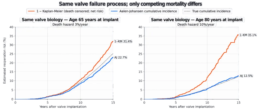
Figure 1. Same valve, same simulated biology. The orange curve (1 − Kaplan–Meier, death censored) estimates net failure and is therefore almost identical in the two cohorts. In this simulation the latent reoperation time is independent of death, so it also lies close to the explicitly simulated risk in a world without death. The blue curve (Aalen–Johansen) tracks the true observed-world cumulative incidence (dashed) and shows how many patients are actually reoperated before death.
Three observations.
1 − KM estimates a net failure quantity, not the observed patient-level cumulative incidence. In both cohorts, 1 − KM lands close to the latent 34% at 15 years because, in this simulation, the latent reoperation time is generated independently of death and is identical in the two cohorts. This is a deliberately favourable setting for the familiar “world without death” interpretation; real clinical data need not satisfy that independence.
The CIF estimates what actually happens in the simulated population. In the 80-year-old cohort, only about one patient in eight is reoperated within 15 years, not one in three. Most patients die before reoperation. Quoting 35% as the observed 15-year probability of reoperation would overstate the population risk almost threefold. For an individual patient, a properly calibrated conditional CIF would still be needed.
Estimates wobble around the truth. At 15 years in the younger cohort, the Aalen–Johansen estimate (22.7%) sits 2 points below the true value. With few patients still at risk at the end of follow-up, that is ordinary sampling variability. Curves should always be reported with confidence intervals and numbers at risk.
Regression: cause-specific versus Fine–Gray
I then fitted both regression models to the pooled data, with age group (80 vs 65) as the only covariate.
| Model | Hazard ratio, age 80 vs 65 | 95% CI |
|---|---|---|
| Cause-specific Cox (death censored) | 1.18 | 0.98–1.42 |
| Fine–Gray (subdistribution) | 0.50 | 0.42–0.60 |
The true cause-specific HR is 1.00, because the valves are identical. The estimate of 1.18 is compatible with it (p = 0.08).
The Fine–Gray model says that older patients have half the subdistribution hazard of reoperation. That is also correct. They really are reoperated much less often. Not because their valves last longer, but because they die first.
Imagine the second number in a registry paper, stripped of context, in a sentence like “older age was independently associated with a lower risk of reoperation (sHR 0.50)”. A reader could easily conclude that bioprostheses are more durable in the elderly. The statement is true about patients and misleading about valves. This is why the question has to come before the model.
6. The code
The simulation uses lifelines (version 0.30.3) [15]. lifelines implements the Aalen–Johansen estimator but not Fine–Gray regression, so the Fine–Gray model was fitted in R with the survival package [16]. As a cross-check, R reproduced the Aalen–Johansen estimates and the cause-specific HR exactly.
Python: simulation, 1 − KM, Aalen–Johansen and cause-specific Cox
import numpy as np
import pandas as pd
from scipy.integrate import quad
from lifelines import KaplanMeierFitter, AalenJohansenFitter, CoxPHFitter

rng = np.random.default_rng(2026)

# 1. Data-generating mechanism ------------------------------------------
WEIBULL_SHAPE, WEIBULL_SCALE = 3.0, 20.0          # latent time to SVD reoperation (years)
MORTALITY = {"65 years": 0.03, "80 years": 0.10}  # constant annual death hazard
N_PER_COHORT = 1500

def simulate_cohort(n, death_rate, label):
    t_reop = WEIBULL_SCALE * rng.weibull(WEIBULL_SHAPE, n)   # latent reoperation time
    t_death = rng.exponential(1 / death_rate, n)             # latent death time
    t_admin = rng.uniform(10, 20, n)                         # staggered entry
    t_lost = rng.exponential(1 / 0.01, n)                    # 1%/year lost to follow-up
    t_cens = np.minimum(t_admin, t_lost)

    time = np.minimum.reduce([t_reop, t_death, t_cens])
    event = np.select([time == t_reop, time == t_death], [1, 2], default=0)
    return pd.DataFrame({"time": time, "event": event, "cohort": label})

df = pd.concat([simulate_cohort(N_PER_COHORT, mu, lab) for lab, mu in MORTALITY.items()],
               ignore_index=True)

# 2. True CIF: integral of h1(u) * S(u), with S(u) = exp(-H1(u) - mu*u) ----
def true_cif(t, mu, k=WEIBULL_SHAPE, lam=WEIBULL_SCALE):
    h1 = lambda u: (k / lam) * (u / lam) ** (k - 1)
    S = lambda u: np.exp(-((u / lam) ** k) - mu * u)
    return quad(lambda u: h1(u) * S(u), 0, t)[0]

def latent_risk(t, k=WEIBULL_SHAPE, lam=WEIBULL_SCALE):
    return 1 - np.exp(-((t / lam) ** k))       # reoperation risk in a world without death

# 3. Estimation -----------------------------------------------------------
rows = []
for label, mu in MORTALITY.items():
    d = df[df.cohort == label]
    km = KaplanMeierFitter().fit(d.time, event_observed=(d.event == 1))   # death censored
    aj = AalenJohansenFitter(seed=2026).fit(d.time, d.event, event_of_interest=1)
    for t in (10, 15):
        rows.append({
            "cohort": label, "year": t,
            "1-KM": 1 - km.survival_function_at_times(t).iloc[0],
            "AJ CIF": aj.cumulative_density_.loc[:t].iloc[-1, 0],
            "true CIF": true_cif(t, mu),
            "latent": latent_risk(t),
        })
print((pd.DataFrame(rows).set_index(["cohort", "year"]) * 100).round(1))

# 4. Cause-specific Cox for reoperation (death censored) -------------------
df["age80"] = (df.cohort == "80 years").astype(int)
df["reop"] = (df.event == 1).astype(int)
cs = CoxPHFitter().fit(df[["time", "reop", "age80"]], "time", "reop")
print(cs.summary[["exp(coef)", "exp(coef) lower 95%", "exp(coef) upper 95%"]].round(2))

df[["time", "event", "cohort"]].to_csv("valve_sim.csv", index=False)Two practical notes. AalenJohansenFitter requires unique event times and adds a tiny random jitter when ties are present; fixing the seed keeps the output reproducible. And the event column must use one code per event type (here 0 = censored, 1 = reoperation, 2 = death), which is also how you should structure your own registry extracts.
Plotting 1 − KM against the CIF
import matplotlib.pyplot as plt

fig, axes = plt.subplots(1, 2, figsize=(12, 5), sharey=True)
for ax, (label, mu) in zip(axes, MORTALITY.items()):
    d = df[df.cohort == label]
    km = KaplanMeierFitter().fit(d.time, event_observed=(d.event == 1))
    aj = AalenJohansenFitter(seed=2026).fit(d.time, d.event, event_of_interest=1)
    (1 - km.survival_function_.loc[:15]).mul(100).plot(ax=ax, drawstyle="steps-post",
                                                       label="1 − Kaplan–Meier")
    aj.cumulative_density_.loc[:15].mul(100).plot(ax=ax, drawstyle="steps-post",
                                                  label="Aalen–Johansen CIF")
    ax.set_title(f"Age {label}")
    ax.set_xlabel("Years after implantation")
axes[0].set_ylabel("Reoperation for SVD (%)")
axes[0].legend()
plt.tight_layout()
plt.show()R: Fine–Gray regression on the same data
library(survival)

df <- read.csv("valve_sim.csv")
df$status <- factor(df$event, levels = 0:2, labels = c("censored", "reop", "death"))
df$age80  <- as.integer(df$cohort == "80 years")

# Cause-specific hazard (death censored)
cs <- coxph(Surv(time, event == 1) ~ age80, data = df)

# Fine–Gray: finegray() builds the weighted, expanded dataset
fg_data <- finegray(Surv(time, status) ~ ., data = df, etype = "reop")
fg <- coxph(Surv(fgstart, fgstop, fgstatus) ~ age80, weights = fgwt, data = fg_data)

summary(cs)$conf.int   # HR 1.18 (0.98-1.42)
summary(fg)$conf.int # sHR 0.50 (0.42-0.60)The cmprsk package (cuminc() and crr()) and tidycmprsk offer equivalent functions. The survival vignette on multi-state models and competing risks by Therneau and colleagues is the best practical introduction I know [16].
7. Reading durability papers in 2026
An old debate that never quite closed
Cardiac surgeons argued about “actual versus actuarial” long before most statisticians used the term competing risks. In 1994, analysing 4,910 porcine valves from two centres, Grunkemeier and colleagues showed that actuarial (Kaplan–Meier) estimates of structural deterioration exceeded the actual risk, and that the gap widened with age [6]. They turned the two curves into a nomogram to help choose the age threshold for a biological valve. They later summarized the difference with the memorable subtitle “apples and lemons” [7].
The magnitude can be striking. In a series of biological aortic prostheses from Munich, Kaempchen and colleagues reported 10-year freedom from reoperation in patients over 60 of 79% by Kaplan–Meier versus 90% by cumulative incidence. At 15 years the gap widened to 55% versus 83% [17]. Same patients, same valves, same events. The first number says that almost half of the valves are reoperated by year 15. The second says that fewer than one patient in five is.
Definitions have matured, and so must the statistics
Durability is no longer measured with reoperation alone. The EAPCI/ESC/EACTS consensus of 2017 [18] and VARC-3 in 2021 [19] separate:
- structural valve deterioration (SVD), a haemodynamic and morphological process graded by echocardiography;
- bioprosthetic valve failure (BVF), which includes severe haemodynamic dysfunction, reintervention and valve-related death;
- reintervention, which is a decision, not only a biological event.
That last point deserves attention. In an 85-year-old with a failing valve and severe comorbidity, the heart team may decide not to intervene. The decision not to reintervene is not, by itself, a competing event: unlike death, it does not necessarily make future reintervention impossible. Instead, it reminds us that reintervention is an imperfect proxy for biological valve failure. It requires both valve dysfunction and a clinical decision to treat. Reintervention rates may therefore underestimate biological deterioration particularly in frail patients.
A more complete way to think about durability is as a multi-state process [14]:
No SVD  →  SVD  →  severe valve dysfunction/BVF  →  reintervention
   ↘          ↘                 ↘
                 death from any state
A multi-state model can estimate the probabilities of occupying these different clinical states over time. For most papers that is more machinery than necessary, but conceptually it makes one point very clear: valve deterioration, valve failure, reintervention and death are related events, not interchangeable endpoints.
PARTNER 3 at seven years as a case study
PARTNER 3 randomized low-risk patients to balloon-expandable TAVR or surgical AVR. In the main seven-year report, the primary composite endpoint occurred in 34.6% after TAVR and 37.2% after surgery (HR 0.87, 95% CI 0.70–1.08), and bioprosthetic valve failure was reported as 6.9% versus 7.3% [1].
The dedicated durability analysis published in JAMA Cardiology in 2026 is particularly instructive because it explicitly treated death as a competing risk [2]. In the valve-implant population, the seven-year cumulative incidences were 7.3% versus 7.6% for stage 2/3 SVD-related bioprosthetic valve dysfunction, 6.9% versus 7.5% for all-cause bioprosthetic valve failure, and 6.0% versus 5.5% for aortic-valve reintervention, for TAVR and surgery respectively [2]. The small difference between the 7.3% surgical BVF figure in the main report and 7.5% in the dedicated analysis reflects differences in the specific analysis/reporting populations rather than a general lesson about competing-risk methods.
The statistical approach is appropriate for an observed-world question about patients, but the paper also illustrates why a CIF should never be read in isolation:
- Mortality itself contributes to the CIF. If one treatment arm has more deaths, fewer patients remain able to experience later valve failure. A lower CIF can therefore arise from less valve failure, more competing mortality, or some combination. Showing the cause-specific event processes alongside the CIF helps separate these mechanisms [10].
- Loss to follow-up was asymmetric. Through seven years, 64 surgical patients versus 31 TAVR patients withdrew or were lost to follow-up [2]. Death can be handled as a competing event, but ordinary loss to follow-up is still censoring. If that censoring is related to prognosis, neither Kaplan–Meier nor Aalen–Johansen automatically solves the problem.
- Echocardiographic durability requires an echocardiogram. Of the 671 patients who were alive and still enrolled at seven years, 537 (80.0%) had echocardiographic data available for the durability analysis [2]. The investigators explicitly reported that no adjustment was made for missing data or for the disproportionate withdrawals in the surgical arm.
That last issue deserves a careful distinction. Competing-risk methods solve the problem created by known competing events such as death. They do not solve unknown outcomes caused by missing follow-up. Depending on the estimand and the missingness mechanism, useful approaches may include inverse-probability-of-observation or censoring weighting, multiple imputation under explicit assumptions, joint or multi-state models, and sensitivity analyses for informative missingness. No method can recover missing information without assumptions.
None of this invalidates PARTNER 3. It makes the trial a useful real-world example of a broader rule: a durability percentage is a function of the valve, the patient population, competing mortality, the endpoint definition and the completeness of follow-up, all at once.
8. A checklist for readers and authors
Before you trust a durability curve, or publish one, run through these eight questions.
1. Is there a competing event? For any valve endpoint in adults, death almost always competes. So can transplantation, or conversion to another therapy.
2. What exactly is plotted? “Freedom from reoperation (Kaplan–Meier)” and “cumulative incidence of reoperation” are different quantities and should be labelled as such. The EJCTS/ICVTS guidelines also ask authors to drop the phrase “actuarial survival” and simply write “survival” [4].
3. What is the scientific question? If the focus is the event rate among patients who remain alive and event-free, cause-specific hazards are natural. If the focus is the observed probability of reoperation over time, report the CIF. Fine–Gray can model covariate associations with that CIF directly, but prediction can also be built from models of all cause-specific hazards [10, 20].
4. Are all event types shown? Numbers at risk, events of interest, competing events and censored observations, per arm and per time point. A CIF without the competing events is half a picture.
5. Are endpoints defined by current standards? EAPCI/ESC/EACTS 2017 or VARC-3 for SVD and BVF [18, 19], with an explicit imaging schedule.
6. Is censoring plausibly non-informative? Check follow-up completeness per arm, the reasons for loss, and whether a sensitivity analysis was performed.
7. Does the population match your patient? A CIF is population-specific. A cumulative incidence from 80-year-olds cannot be transported to 60-year-olds, because the competing mortality is different. The same logic applies when you check the calibration of a risk model in a new population.
8. Is a composite endpoint hiding the issue? “Death or reoperation” avoids competing risks by merging them, but it answers yet another question. It is useful for event-free survival, not for durability.
Take-home messages
1. Kaplan–Meier with death censored estimates net failure, not observed cumulative incidence. It can be useful for describing the event-specific failure process, but interpreting it literally as “what would happen if nobody died” requires additional assumptions.
2. The cumulative incidence function estimates the observed-world population probability. With complete follow-up and no ordinary censoring it reduces to the observed proportion. It is the appropriate descriptive quantity for counselling and planning, while individual counselling requires conditional, calibrated prediction.
3. The gap between the two grows with competing mortality. It is modest in young patients and can be threefold in the elderly, precisely the population where transcatheter and biological valves are used most.
4. Cause-specific and Fine–Gray models answer different questions. The same covariate can have a cause-specific HR of 1 and a subdistribution HR of 0.5. Neither estimate is inherently wrong. The important step is to decide whether you want to model an event-specific rate, the cumulative incidence, or an individual absolute risk.
5. Report both sides. Cause-specific hazards for all events, cumulative incidence functions, numbers at risk and follow-up completeness. That is what current methodological guidance and journal statistical guidelines ask for.
Conclusion
When my 78-year-old patient asks how long her valve will last, she is really asking two things. How long will the tissue hold? And will she ever need another operation? The first is a question about pericardium and calcium. The second is a question about her whole life.
Kaplan–Meier with death censored provides a net view of the failure process. The cumulative incidence function answers the observed-world population question: how often reoperation actually occurs before death. Both can belong in a durability paper, provided they are labelled for what they estimate. For the conversation with an individual patient, the most useful number is a conditional, well-calibrated cumulative incidence for someone with her characteristics.
FAQ
Is Kaplan–Meier wrong for valve durability?
No, but it answers a narrower question than many readers assume. With death censored, 1 − KM estimates a net failure quantity rather than the observed cumulative incidence. It is useful for describing the event-specific failure process. Interpreting it literally as the probability in a hypothetical world without death requires additional assumptions.
What is the difference between “actual” and “actuarial” freedom from reoperation?
“Actuarial” is the older surgical term for the Kaplan–Meier estimate, which treats deaths as censored. “Actual” refers to the cumulative incidence, which accounts for death as a competing event. Actual risk is always lower than or equal to actuarial risk.
Why does 1 − Kaplan–Meier overestimate the risk of reoperation?
Because it redistributes the future events of patients who died to those who are still alive, as if the dead were still at risk. The more patients die, the larger the overestimation.
When should I use a Fine–Gray model instead of a cause-specific Cox model?
Use cause-specific Cox models when the target is the event-specific rate among patients who remain event-free. Use Fine–Gray when you want a regression model tied directly to the cumulative incidence. Fine–Gray is not the only way to predict absolute risk: separate cause-specific models for all event types can also be combined to derive a CIF. Methodological guidance recommends showing the cumulative incidence and reporting the relevant cause-specific hazards.
Can I compute cumulative incidence in Python?
Yes. The AalenJohansenFitter in lifelines estimates the CIF. For Fine–Gray regression the reference implementations are in R (survival::finegray, cmprsk::crr, tidycmprsk).
Does a composite endpoint such as “death or reoperation” solve the problem?
It removes the competing risk by merging the events, but it changes the question. Event-free survival is a meaningful endpoint, but it cannot tell you how durable the valve is.
Statistical perspective. This article is an educational explanation of competing risks methods applied to valve durability. The simulation is illustrative and does not describe any real prosthesis or patient population. Clinical decisions should rely on the full published evidence and individualized heart-team assessment.
References
- Leon MB, Mack MJ, Pibarot P, et al. Transcatheter or surgical aortic-valve replacement in low-risk patients at 7 years. N Engl J Med. 2026;394:773-783. doi:10.1056/NEJMoa2509766.
- Ternacle J, Hahn RT, Silva I, et al. Seven-year valve durability with transcatheter or surgical aortic valve replacement: an ad hoc analysis of the PARTNER 3 randomized clinical trial. JAMA Cardiol. 2026;11(8):747-757. doi:10.1001/jamacardio.2026.2299.
- Akins CW, Miller DC, Turina MI, et al. Guidelines for reporting mortality and morbidity after cardiac valve interventions. Eur J Cardiothorac Surg. 2008;33(4):523-528.
- Hickey GL, Dunning J, Seifert B, et al. Statistical and data reporting guidelines for the European Journal of Cardio-Thoracic Surgery and the Interactive CardioVascular and Thoracic Surgery. Eur J Cardiothorac Surg. 2015;48(2):180-193. doi:10.1093/ejcts/ezv168.
- Kaplan EL, Meier P. Nonparametric estimation from incomplete observations. J Am Stat Assoc. 1958;53(282):457-481.
- Grunkemeier GL, Jamieson WR, Miller DC, Starr A. Actuarial versus actual risk of porcine structural valve deterioration. J Thorac Cardiovasc Surg. 1994;108(4):709-718.
- Grunkemeier GL, Jin R, Eijkemans MJ, Takkenberg JJ. Actual and actuarial probabilities of competing risks: apples and lemons. Ann Thorac Surg. 2007;83(5):1586-1592. doi:10.1016/j.athoracsur.2006.11.044.
- Andersen PK, Geskus RB, de Witte T, Putter H. Competing risks in epidemiology: possibilities and pitfalls. Int J Epidemiol. 2012;41(3):861-870.
- Aalen OO, Johansen S. An empirical transition matrix for non-homogeneous Markov chains based on censored observations. Scand J Stat. 1978;5(3):141-150.
- Latouche A, Allignol A, Beyersmann J, Labopin M, Fine JP. A competing risks analysis should report results on all cause-specific hazards and cumulative incidence functions. J Clin Epidemiol. 2013;66(6):648-653.
- Wolbers M, Koller MT, Stel VS, et al. Competing risks analyses: objectives and approaches. Eur Heart J. 2014;35(42):2936-2941.
- Austin PC, Lee DS, Fine JP. Introduction to the analysis of survival data in the presence of competing risks. Circulation. 2016;133(6):601-609.
- Fine JP, Gray RJ. A proportional hazards model for the subdistribution of a competing risk. J Am Stat Assoc. 1999;94(446):496-509.
- Putter H, Fiocco M, Geskus RB. Tutorial in biostatistics: competing risks and multi-state models. Stat Med. 2007;26(11):2389-2430.
- Davidson-Pilon C. lifelines: survival analysis in Python. J Open Source Softw. 2019;4(40):1317.
- Therneau T, Crowson C, Atkinson E. Multi-state models and competing risks. Vignette of the R package survival. Comprehensive R Archive Network.
- Kaempchen S, Guenther T, Toschke M, Grunkemeier GL, Wottke M, Lange R. Assessing the benefit of biological valve prostheses: cumulative incidence (actual) vs. Kaplan–Meier (actuarial) analysis. Eur J Cardiothorac Surg. 2003;23(5):710-714.
- Capodanno D, Petronio AS, Prendergast B, et al. Standardized definitions of structural deterioration and valve failure in assessing long-term durability of transcatheter and surgical aortic bioprosthetic valves: a consensus statement from the EAPCI endorsed by the ESC and EACTS. Eur Heart J. 2017;38(45):3382-3390.
- VARC-3 Writing Committee; Généreux P, Piazza N, Alu MC, et al. Valve Academic Research Consortium 3: updated endpoint definitions for aortic valve clinical research. Eur Heart J. 2021;42(19):1825-1857.
- Austin PC, Fine JP. Practical recommendations for reporting Fine-Gray model analyses for competing risk data. Stat Med. 2017;36(27):4391-4400. doi:10.1002/sim.7501.
- Young JG, Stensrud MJ, Tchetgen Tchetgen EJ, Hernán MA. A causal framework for classical statistical estimands in failure-time settings with competing events. Stat Med. 2020;39(8):1199-1236. doi:10.1002/sim.8471.