Statistical Distributions

Introduction

Statistical distributions represent the modes observed for each statistical unit. It is also a mathematical model describing how a variable’s values are distributed within a population or sample.

Expressed in this “classic” way, the concept is somewhat unclear, but some examples can help clarify it.

Imagine a bag filled with candies of various flavors. If we count the number of candies for each flavor and present the results in a table, we have a statistical distribution.

Flavor	Number of candies
Strawberry	10
Lemon	5
Mint	3
Licorice	12
Blackberry	5

Another example is the distribution of grades obtained by a group of students in a test. Suppose we have 5 students scoring 7, 10 students scoring 8, and 5 students scoring 9. The resulting statistical distribution is:

Grade	7	8	9
Number of students	5	10	5

Essentially, a statistical distribution is a method to organize and visualize data, allowing us to better understand how different values are spread out.

The simple unitary statistical distribution is the list of modes observed for each statistical unit.

For students who have taken a test, it can be organized as follows:

Student (statistic unit)	Grade (observed mode)
Mary	7
Michael	9
James	7
Jennifer	8
…	…

The absolute frequency distribution is created by showing the number of units where a specific mode is observed:

Grade (observed mode)	7	8	9
Number of students (with the corresponding number of occurrences)	5	10	5

The relative frequency distribution represents the ratio of the number of units with the observed mode to the total number of statistical units:

Grade (observed mode)	7	8	9
Relative Frequence	5/20 = 0.25 = 25%	10/20 = 0.5 = 50%	5/20 = 0.25 = 25%

---

General Formula for Statistical Distributions

There exists a multitude of different statistical distributions due to several factors:

• Variety of phenomena: Different natural and social processes produce data with unique characteristics;
• Mathematical properties: Some distributions have properties that make them ideal for modeling specific types of data;
• Application contexts: Some distributions are better suited to specific fields or types of analysis.

Distributions are categorized as discrete or continuous based on the type of variable they represent. Discrete distributions are typically presented using tables or bar charts, while continuous distributions are best illustrated with curves.

To identify the distribution type, a general formula is used and then tailored for each specific distribution:

X is a random variable

~ (tilde) is read as “is distributed as”

N represents the type of distribution. (Usually, N stands for Normal Distribution)

In parentheses are the parameters of the distribution. These typically include quantities such as the mean, variance, standard deviation, shape parameters, and rate parameters, depending on the specific type of distribution.

In summary, when we write X ~ N(mu, sigma square), we’re stating that the random variable X follows a normal distribution with mean mu and variance sigma^2. This notation succinctly describes X’s probabilistic behavior, enabling us to calculate probabilities for specific ranges of X.

---

Discrete distributions

Uniform distribution

X ~ U (a,b)

The uniform distribution maintains a constant probability across its entire interval. Parameters a and b denote the lower and upper limits, respectively.

A visual representation of a uniform distribution can be generated using Python:

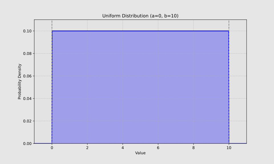
The uniform distribution is applicable in scenarios like patient randomization. When selecting cases from a database using this distribution, each patient has an equal chance of being chosen.

Generally, the uniform distribution is less common, particularly in medical contexts where more complex distributions are prevalent.

Bernoulli Distribution

X ~ Bern (p)

The Bernoulli distribution is a discrete probability distribution that models a single experiment with only two possible outcomes (for example, success and failure). Here, p represents the probability of success.

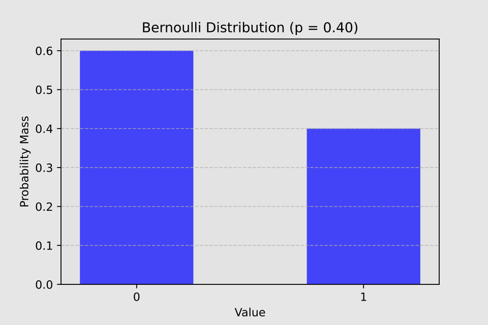
Examples of Bernoulli distribution in the medical field:

• Therapy response in a single patient (positive or negative outcome)
• Single diagnostic test result for a patient (positive or negative)
• Post-intervention survival of a patient (alive or deceased)

The Bernoulli distribution serves as the foundation for a more sophisticated distribution: the binomial distribution.

Binomial distribution

X ~ B (n, p)

When we repeat n independent Bernoulli trials, each with the same probability of success, we obtain a binomial distribution.

The distribution’s parameters are n and p: n represents the number of trials, while p denotes the probability of success.

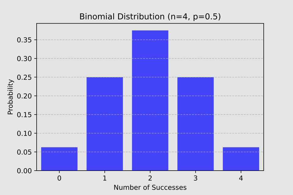
Examples of binomial distribution:

• Treatment of 100 patients with a drug having a 60% success probability: B(100, 0.6)
• Side effect occurrence in 1000 patients taking a drug with a 5% probability: B(1000, 0.05)

The binomial distribution plays a crucial role in clinical research. One of its notable features is that when the number of trials exceeds 30 and the probability approaches 0.5, its distribution can be approximated by a normal distribution.

Poisson Distribution

X ~ Poisson (λ)

The Poisson distribution models the occurrence of events within a fixed time interval or spatial area.

λ (lambda) represents the average rate of occurrence.

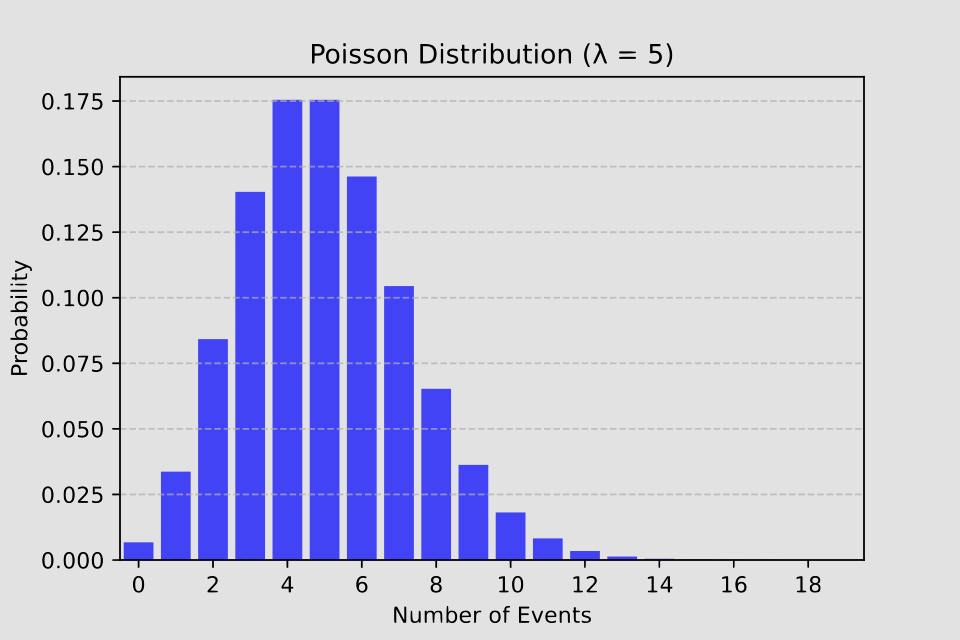
Examples of Poisson distribution:

• Emergency room arrivals in one hour. If 5 patients arrive per hour, it can be configured as Poisson(5)
• Nosocomial infections in a ward in a month
• The number of calls to emergency services in 24 hours

The Poisson distribution is especially useful for modeling rare events. However, it’s important to note that this distribution assumes events are independent and occur at a constant average rate. In reality, particularly in healthcare settings, these assumptions may not always be valid.

---

Continuous distributions

Normal distribution

X ~ N (µ, σ ²)

This distribution, also known as Gaussian, is one of the most important and widely used in statistics. It’s characterized by its distinctive symmetrical bell-shaped curve.

µ (mu) represents the mean and σ² (sigma squared) denotes the variance.

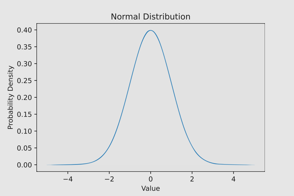
The normal distribution’s symmetrical nature allows for a useful rule of thumb known as the 68-95-99.7 rule. This rule states that:

• Approximately 68% of the data falls within one standard deviation of the mean • About 95% of the data is contained within two standard deviations of the mean • Nearly 99.7% of all data points lie within three standard deviations of the mean

This principle is particularly valuable in statistics and data analysis, as it provides a quick way to understand the spread of data in a normal distribution without complex calculations.

There are numerous medical parameters within a population that exhibit a normal distribution. This statistical pattern is observed in various physiological measurements, including:

1. Blood pressure: both systolic and diastolic readings tend to follow a normal distribution in large populations.
2. Body Mass Index (BMI): the distribution of BMI values across a population often approximates a normal curve.
3. Cholesterol levels: total cholesterol, as well as specific types like HDL and LDL, typically show a normal distribution.
4. Height and weight: these anthropometric measurements generally follow a normal distribution when assessed across a large, diverse population.
5. Hemoglobin levels: In healthy individuals, hemoglobin concentrations often display a normal distribution.
6. White blood cell counts: the number of white blood cells in healthy individuals tends to follow a normal distribution pattern.

These normally distributed parameters are valuable in clinical practice and research, as they allow for the establishment of reference ranges and the identification of potential health issues when individual measurements deviate significantly from the population norm.

Student’s t-distribution

X ~t (ν)

The Student’s t-distribution, a continuous probability distribution, is particularly valuable when analyzing small datasets or when the population variance is unknown. It finds extensive application in medical research and statistical analysis.

The parameter ν (nu) represents the degrees of freedom (df). As the df increases, the t-distribution curve gradually approaches that of a normal distribution.

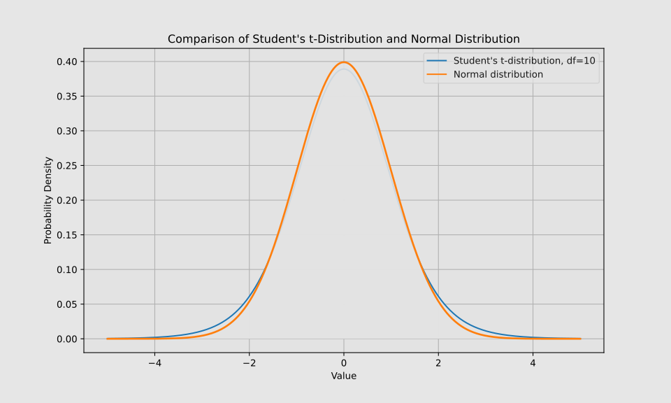
Visually, the Student’s t-distribution shares similarities with the normal distribution, but is characterized by more pronounced tails. This distinctive feature makes the t-distribution an indispensable tool in statistical analysis. Its significance lies in its ability to facilitate accurate inferences from limited data sets, even when working with small sample sizes. Moreover, the t-distribution demonstrates a notable level of resilience, maintaining its reliability even in scenarios where the assumption of normality is not strictly adhered to. This robustness makes it particularly valuable in real-world applications where data may not always conform perfectly to theoretical ideals.

Chi-square distribution

N~X²(k)

The parameter k denotes the degrees of freedom.

The chi-square distribution curve is right-skewed and always positive.

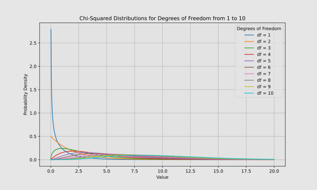
This distribution is widely used in clinical research for various purposes:

• Assessing the effectiveness of treatments
• Analyzing relationships between potential risk factors and diseases through contingency tables
• Evaluating the homogeneity of effects across different studies in meta-analyses
• Comparing survival curves

A key strength of the chi-square distribution is its applicability to categorical data, which is prevalent in clinical studies.

However, it’s important to note that this distribution requires sufficiently large sample sizes for reliable results.

Exponential distribution

X ~ Exp(λ)

The exponential distribution is a continuous probability model that describes the time until an event occurs, assuming the event has a constant probability of happening at any given moment.

The parameter λ (lambda) represents the average rate at which the event occurs. As previously noted, this rate must remain constant for the distribution to apply.

The exponential distribution’s graph is characterized by a steep curve that starts high and rapidly declines, forming an extended “tail” that asymptotically approaches but never intersects the horizontal axis.

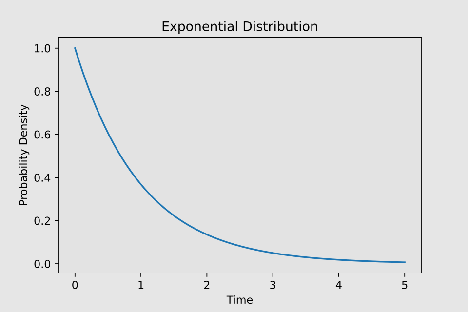
In medicine, certain phenomena—such as drug concentration decay in the body or disease distribution patterns—exhibit exponential trends. However, in practice, these phenomena often deviate from a simple exponential distribution, assuming more complex patterns that require alternative models for accurate representation.

Logistic distribution

This distribution, also known as the logistic function or S-curve, is a mathematical model used to describe population growth or the spread of a phenomenon over time. The S-curve depicts an initial slow growth phase, followed by rapid acceleration, and then another slow growth phase.

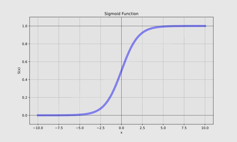
The logistic distribution has numerous applications in medicine. It can model the spread of infectious diseases like influenza in a population. The infection rate typically starts slow, accelerates rapidly as more people become infected, then slows down as the pool of susceptible individuals shrinks. Surgeons’ learning curves for new procedures often mirror this pattern: initial slow improvement, followed by rapid skill acquisition, and finally a plateau as they approach mastery. In pharmacology, drug efficacy often follows a logistic curve as dosage increases. At low doses, the effect may be minimal. It then increases rapidly within a certain range before leveling off at higher doses, often due to saturation of drug receptors or other physiological limits.

Further Readings

DataScience Dojo

Khan academy

Conclusions

Statistical distributions are fundamental tools for understanding and analyzing data patterns, ranging from simple discrete models like Bernoulli and binomial distributions to more complex continuous distributions like normal and logistic. Each distribution type serves specific purposes in statistical analysis, particularly in medical and research contexts. Understanding these distributions is crucial for proper data interpretation and statistical inference, especially in clinical research and healthcare settings where they inform decision-making and help establish meaningful reference ranges.

---

For those interested in creating these distribution curves using Python, refer to the post “Visualizing Statistical Distributions with Python”.