
Note: You can find additional posts about linear regression elsewhere on this site that offer a machine learning perspective.
Introduction to Linear Regression
Unlike correlation, which examines the relationship between two variables without identifying a cause-effect link, linear regression relates a dependent variable (usually denoted as Y) to one or more independent variables (X₁, X₂… Xₙ).
What Is Linear Regression?
Linear regression assumes that the relationship between independent and dependent variables follows a linear trend—one that a straight line can represent.
To simplify, let’s focus on the relationship between two variables: one dependent and one independent. We can create a graph plotting the X and Y values as points. The goal is to find a line that best fits these points, often only approximately.
Since many lines can be drawn, we choose the one with the smallest distance between the actual values and the points that fall on the line.
The distance between an actual data point and the regression line is called a “residual” or “error.”
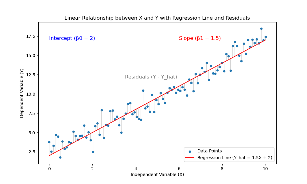
Minimizing the errors
The sum of squared errors (SSE) is calculated by adding up all these squared residuals. Squaring emphasizes larger deviations because bigger distances, when squared, increase the sum more significantly. This approach penalizes lines with larger errors compared to those with lower SSE.
$\text{SSE} = \sum_{i=1}^n (Y_i – \hat{Y}_i)^2$
We use the Ordinary Least Squares (OLS) method to find the best-fitting line. This method selects the line with the lowest SSE from all possible options. For simple regression, the OLS method identifies two coefficients of the regression line: β0 for the intercept and β1 for the slope.
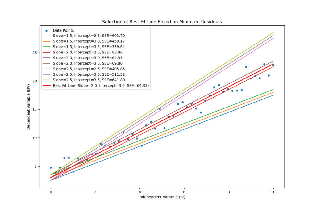
The process culminates in an equation for a line that best represents the relationship between the two variables (i.e., with the smallest residuals or errors):
$Y = \beta_0 + \beta_1 X + \epsilon$
Linear regression is called simple when examining the relationship between one independent variable and the dependent variable, and multiple when analyzing relationships between several independent variables and the dependent variable. In this case the equation expands to:
$Y = \beta_0 + \beta_1 X_1 + \beta_2 X_2 + \dots + \beta_n X_n + \epsilon$
In these equations:
- Y is the dependent variable
- X represents the independent variable(s)
- β0 is the y-intercept—the predicted value of Y when X equals zero
- β1 (and subsequent β coefficients) represent the slope, indicating how much Y is expected to change for each unit increase in X
- ϵ is the error term, showing the difference between observed and predicted values
Multiple linear regression incorporates several βX pairs, one for each independent variable in the equation.
Assumptions of Linear Regression
- Linearity: A linear relationship must exist between the variables. When graphing the dependent and independent variables, the points should roughly follow a linear trend.
- Independence of errors: The errors (or residuals) must be independent of each other.
- Homoscedasticity: The variance of errors should remain constant for all values of X.
- Normality of errors: The errors must follow a normal distribution.
- Absence of multicollinearity: The independent variables should not be strongly correlated with each other.
Results
A simple linear regression analysis yields a comprehensive set of statistical information, offering insights into the relationship between variables.
Key results include coefficients for the constant (intercept) and slope, along with their standard errors—indicators of estimate precision. T-statistics help determine if these coefficients significantly differ from zero, while confidence intervals support interpretation.
The R-squared (R²) value is a crucial metric. This coefficient of determination, expressed as a percentage, reveals the proportion of variance in the dependent variable explained by the independent variable. An adjusted R² is also provided, accounting for the number of independent variables and sample size, offering a more conservative estimate of the model’s explanatory power. The F-statistic evaluates the overall goodness of fit of the regression model.
To validate the regression analysis, diagnostic statistics are included. The Durbin-Watson statistic detects autocorrelation in residuals, which could violate a key assumption of linear regression. The Omnibus test assesses whether residuals follow a normal distribution—another crucial assumption. These statistics help verify that the model meets necessary assumptions, ensuring reliable results.
Simple Linear Regression in Python
Let’s create a sample dataset to analyze a simple linear regression and present the results.
import numpy as np
import statsmodels.api as sm
import matplotlib.pyplot as plt

# Generate synthetic data
np.random.seed(0)
X = np.linspace(0, 10, 50)
true_slope = 2
true_intercept = 3
noise = np.random.normal(0, 1, X.shape)
Y = true_slope * X + true_intercept + noise

# Perform regression
X_with_intercept = sm.add_constant(X)
model = sm.OLS(Y, X_with_intercept)
results = model.fit()

# Plot data points and regression line
plt.figure(figsize=(12, 8))
plt.scatter(X, Y, label="Data Points")
plt.plot(X, results.predict(X_with_intercept), color="red", label="Regression Line")
plt.xlabel("Independent Variable (X)")
plt.ylabel("Dependent Variable (Y)")
plt.title("Linear Regression with Summary")

# Create a separate figure for the summary text
fig, ax = plt.subplots(figsize=(10, 6))
ax.axis('off')  # Remove axes
summary_text = results.summary().as_text()
plt.text(0.01, 0.99, summary_text, transform=plt.gca().transAxes, fontsize=10, family="monospace", ha="left", va="top")

# Display both plots
plt.show()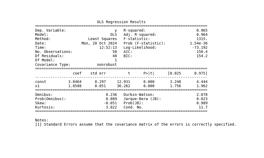
Multiple Linear Regression in Python
In multiple linear regression, each independent variable is assigned its own coefficient, t-statistic, and p-value.
The model’s overall performance is assessed using R², adjusted R², and an F-statistic—all of which carry the same interpretation as in single-variable models. Additionally, the model’s adherence to underlying assumptions is evaluated.
Let’s create a fictional dataset to examine a multiple linear regression and analyze its results.
import pandas as pd
import numpy as np
import statsmodels.api as sm
import matplotlib.pyplot as plt

# Seed for reproducibility
np.random.seed(42)

# Generate synthetic data for a multiple linear regression scenario with medical context
n_samples = 100
age = np.random.randint(20, 80, n_samples)  # Age of patients
bmi = np.random.uniform(18, 35, n_samples)  # BMI of patients
blood_pressure = 0.5 * age + 0.3 * bmi + np.random.normal(0, 5, n_samples)  # Outcome: Blood Pressure

# Prepare the data in a DataFrame
data = pd.DataFrame({
    "Age": age,
    "BMI": bmi,
    "Blood_Pressure": blood_pressure
})

# Define dependent and independent variables
X = data[["Age", "BMI"]]
Y = data["Blood_Pressure"]
X = sm.add_constant(X)  # Add intercept

# Perform the multiple linear regression
model = sm.OLS(Y, X)
results = model.fit()

# Summary and visualizations
# Plotting data points and regression summary
fig, ax = plt.subplots(figsize=(10, 6))
ax.axis('off')  # Turn off axes for summary text display
summary_text = results.summary().as_text()

# Display summary text on the plot
plt.text(0.01, 0.99, summary_text, transform=ax.transAxes, fontsize=10, family="monospace", ha="left", va="top")
plt.show()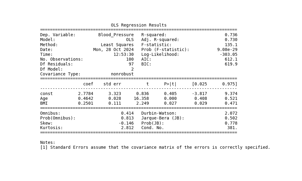
Applications of Linear Regression in Medicine
In the medical field, linear regression finds applications in numerous areas, such as:
- Predicting physiological parameters
- Developing pharmacokinetic and pharmacodynamic models
- Conducting epidemiological or population studies
- Analyzing medical images
Conclusion
Linear regression is a powerful tool for analyzing relationships between variables, but it requires that certain assumptions are met. When these assumptions are violated and corrections aren’t feasible, several alternatives exist. These include logistic regression, polynomial regression, non-linear models, robust regression, principal component analysis (PCA), ridge or lasso regression, and mixed-effects models.
Two techniques deserve a closer look when working with small clinical datasets: cubic splines, which relax the linearity assumption without abandoning the regression framework, and bootstrap validation, which gives a more honest estimate of model performance than a single train/test split.