UNet

Introduction

UNet is a convolutional neural network (CNN) introduced by Olaf Ronneberger in 2015. These specialized neural networks learn to recognize objects in images. When properly trained, they can analyze medical images, detect specific features (such as neoplasms in CT scans), and classify different types of images (such as distinguishing between pneumonia and neoplasms).

In particular, UNet performs semantic interpretation of images by identifying and classifying pixels. It was specifically designed for medical applications and has the advantage of working effectively with small datasets.

UNet Anatomy

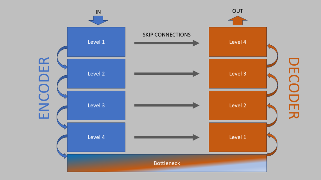
The UNet architecture consists of two joined arms that form a U-like shape: a left Encoder arm that extracts significant features from an image, and a right Decoder arm that reconstructs the image using the extracted information. Skip Connections between the arms link corresponding layers of the Encoder and Decoder, helping maintain spatial details.

Encoder Structure

The encoder consists of 4 levels. Each level includes:

two Convolutional Blocks
a Max Pooling layer
a channel multiplier (filter)

Level of Encoder

The first convolutional block examines images pixel by pixel to detect patterns like corners and shapes. They do this by sliding a 3 × 3 filter (kernel) across the image, multiplying pixel values by filter weights and summing the results at each position.

The first convolutional block applies sixty-four 3×3 filters to the image.

This process creates a “feature map” that summarizes all recognized patterns in the image.

For example, when searching for edges and lines, they will be highlighted in the feature map once the convolutional block is processed.

After convolution, a ReLU (Rectifier Linear Unit) function is applied that converts all negative values to 0 while preserving positive values.

The second convolutional block repeats this process with another filter, creating more complex structures from the patterns identified in the first block. For instance, while the first block detects edges and lines, the second block combines these elements into shapes like circles and rectangles.

After the second convolutional block, the Max Pooling layer reduces the dimensions by 50%.

Through this process, the initial 572 × 572 pixel image is transformed by 64 3 × 3 filters into a 570 × 570 × 64 array. The second convolution with a 3 × 3 filter transforms the image to 568 × 568 pixels, and then the Max Pooling reduces it to 284 × 284 × 64 before proceeding to the next block.

Subsequent Encoder Levels

Through this process, at the first level of Encoder the initial 572 × 572 pixel image is transformed by 64 3 × 3 filters into a 570 × 570 × 64 array. The second convolution with a 3 × 3 filter transforms the image to 568 × 568 pixels, and then the Max Pooling reduces it to 284 × 284 × 64 before proceeding to the next block.

The subsequent levels (second, third, and fourth) mirror the first level’s structure. Each consists of two successive 3 × 3 convolutional blocks followed by Max Pooling. As each convolutional block introduces new filters, this process progressively reduces the image’s pixel dimensions while increasing the number of channels (filters).

Summary of Encoder Modifications

(Starting with a 572 × 572 × 1 grayscale image)

Level	Operation	Channel	Image Pixel
I	2 convolutional block 3×3 and 1 max pooling 2 x2	64	572 x 572
	2 convolutional block 3×3 and 1 max pooling 2 x2	128	284 x 284
III	2 convolutional block 3×3 and 1 max pooling 2 x2	256	140 x 140
IV	2 convolutional block 3×3 and 1 max pooling 2 x2	512	70 x 70 to 34 x 34

As the image progresses through different levels, its content becomes increasingly abstract and concentrated. At the first level, the network detects simple features like edges and corners. These basic elements combine into shapes at the second level, evolve into more complex structures (such as textures and object parts) at the third level, and finally transform into overall semantic meaning at the fourth level. This increasing complexity corresponds directly with the growing number of channels.

Bottleneck

The bottleneck serves as the final part of the Encoder process and bridges the Encoder and Decoder. It receives the minimally reduced image with maximum channels from the Encoder and applies two additional 3 × 3 convolutional blocks without Max Pooling before transferring it to the Decoder.

During this process, the number of channels increases to 1024.

At this stage, the image reaches its most compressed form.

The first convolutional block reduces the image to 32 × 32 pixels, while the second block further compresses it to 30 × 30 pixels.

The final Bottleneck output is a 30 × 30 pixel image with 1024 channels.

Level of Decoder

The Decoder, which forms UNet’s “ascending” branch, consists of 4 identical blocks.

Each block performs a sequence of operations: upsampling, concatenation, and two convolutions.

Upsampling increases the feature map dimensions from the Bottleneck’s minimum 30 × 30 pixels. This process uses a 2 × 2 transposed convolution kernel to expand the dimensions. In the first block, upsampling takes a 30 × 30 pixel image with 1024 channels and produces a 62 × 62 pixel image with 514 channels.

Upsampling serves two main purposes:

It reconstructs images by recovering details lost during the encoder process
It aligns the feature map dimensions with the corresponding encoder level to enable concatenation via skip connections

After upsampling, the image is concatenated with its corresponding image from the homologous encoder block through the skip connection, joining them along the channel dimension.

The image from the last Encoder block (70 × 70 × 514 channels) is cropped to match the Decoder’s dimensions.

The dimensions combine as follows:

62 x 62 x 514 (Encoder) + 62 x 62 x 514 (Decoder) = 62 x 62 x 1024

Finally, the concatenated image undergoes two 3 × 3 convolutions, reducing it to the first decoder level’s output dimensions of 62 × 62 × 514.

Subsequent Decoder Levels

If the first level, with upsampling operations, concatenation and double convolution brings the image from the bottleneck to dimensions of 62 x 62 x 514, in the subsequent Decoder levels, all identical, the images are increased until reaching final dimensions of 464 x 464 x 64 at the end of the last stage

Summary of Decoder Modifications

LEVEL	1	2	3	4
DECODER INPUT	30×30×1024	58×58×512	116×116×256	232×232×128
UPSAMPLING	62×62×512	120×120×256	236×236×128	468×468×64
SKIP CONNECTION	62×62×512	120×120×256	236×236×128	468×468×64
CONCATENATION	62×62×1024	120×120×512	236×236×256	468×468×128
AFTER CONVOLUTIONS	58×58×512	116×116×256	232×232×128	464×464×64

After the final Decoder stage, the network applies a 1×1 convolution followed by an activation function (either SoftMax or sigmoid) to calculate the probability for each pixel.

The final output is a 464×464 image.

Architectural Overview

INPUT: 572x572x1
│
├── Encoder
│   ├── Conv(3x3, 64) → ReLU → Conv(3x3, 64) → ReLU → MaxPool(2x2)
│   ├── Conv(3x3, 128) → ReLU → Conv(3x3, 128) → ReLU → MaxPool(2x2)
│   ├── Conv(3x3, 256) → ReLU → Conv(3x3, 256) → ReLU → MaxPool(2x2)
│   └── Conv(3x3, 512) → ReLU → Conv(3x3, 512) → ReLU → MaxPool(2x2)
│
├── Bottleneck
│   └── Conv(3x3, 1024) → ReLU → Conv(3x3, 1024) → ReLU → UpConv(2x2)
│
└── Decoder
    ├── Concatenate(UpConv, Encoder[4]) → Conv(3x3, 512) → ReLU → Conv(3x3, 512) → ReLU → UpConv(2x2)
    ├── Concatenate(UpConv, Encoder[3]) → Conv(3x3, 256) → ReLU → Conv(3x3, 256) → ReLU → UpConv(2x2)
    ├── Concatenate(UpConv, Encoder[2]) → Conv(3x3, 128) → ReLU → Conv(3x3, 128) → ReLU → UpConv(2x2)
    └── Concatenate(UpConv, Encoder[1]) → Conv(3x3, 64) → ReLU → Conv(3x3, 64) → ReLU
│
└── Output: Conv(1x1, C) → Sigmoid/Softmax

INPUT: 572x572x1
│
├── Encoder
│   ├── Conv(3x3, 64) → ReLU → Conv(3x3, 64) → ReLU → MaxPool(2x2)
│   ├── Conv(3x3, 128) → ReLU → Conv(3x3, 128) → ReLU → MaxPool(2x2)
│   ├── Conv(3x3, 256) → ReLU → Conv(3x3, 256) → ReLU → MaxPool(2x2)
│   └── Conv(3x3, 512) → ReLU → Conv(3x3, 512) → ReLU → MaxPool(2x2)
│
├── Bottleneck
│   └── Conv(3x3, 1024) → ReLU → Conv(3x3, 1024) → ReLU → UpConv(2x2)
│
└── Decoder
    ├── Concatenate(UpConv, Encoder[4]) → Conv(3x3, 512) → ReLU → Conv(3x3, 512) → ReLU → UpConv(2x2)
    ├── Concatenate(UpConv, Encoder[3]) → Conv(3x3, 256) → ReLU → Conv(3x3, 256) → ReLU → UpConv(2x2)
    ├── Concatenate(UpConv, Encoder[2]) → Conv(3x3, 128) → ReLU → Conv(3x3, 128) → ReLU → UpConv(2x2)
    └── Concatenate(UpConv, Encoder[1]) → Conv(3x3, 64) → ReLU → Conv(3x3, 64) → ReLU
│
└── Output: Conv(1x1, C) → Sigmoid/Softmax

UNet Results

UNet generates a “segmentation map” (called a Mask) rather than returning a copy of the input image. This Mask highlights structures of interest by assigning numerical values to each pixel.

The Mask maintains the same dimensions as the original image, with pixel values varying based on the classification task:

In binary classification, pixels get a value of 1 for the structure of interest and 0 for everything else
In multiclass classification, pixels receive values corresponding to their class (1 for the first class, 2 for the second class, 0 for background)

For example, when UNet is trained to detect tumors, the Mask marks tumor pixels with 1 and non-tumor pixels with 0.

We can visualize the tumor’s location by overlaying this mask on the original image.

UNet Evaluation Metrics

The quality of results obtained by UNet can be evaluated using different metrics:

Dice Coefficient

The Dice Coefficient can be compared to the F1 score for images.

A Dice Coefficient equal to one indicates a perfect map.

Considering P as the predicted map and G as the ground truth map, the dice coefficient is:

$\text{Dice} = \frac{2 \cdot |P \cap G|}{|P| + |G|}$

Intersection over Union (IoU)

Another metric is the Intersection over Union which also classifies a perfect map as 1. Unlike the Dice coefficient, IoU (Jaccard Index) is more sensitive to small differences

$\text{IoU} = \frac{|P \cap G|}{|P \cup G|} = \frac{|P \cap G|}{|P| + |G| - |P \cap G|}$

Accuracy

Measures the percentage of correctly classified pixels

Precision/recall

Ability to recognize true positives without false positives.

Challenges When Using UNet

The first challenge is dimensional discrepancy between input and output images. Without proper corrections, the output image becomes smaller than the input. This can be resolved by applying padding to the convolutions or by upscaling the final result.

The second challenge is overfitting, where the model becomes too specialized to its training examples. This is addressed through data augmentation techniques.

The third challenge is class imbalance, particularly common in biomedical data. For instance, a tumor might occupy only a small portion of the image’s pixels. To handle this, specialized loss functions like Dice Loss or Focal Loss are implemented.

Applications of UNet in Medicine

There are examples of UNet applications in the medical field:

Walsh J – Using U-Net network for efficient brain tumor segmentation in MRI images – https://doi.org/10.1016/j.health.2022.100098**

Hassanpour N, Deep Learning-based Bio-Medical Image Segmentation using UNet Architecture and Transfer Learning – https://doi.org/10.48550/arXiv.2305.14841

Ehab W – Performance Analysis of UNet and Variants for Medical Image Segmentation – https://doi.org/10.48550/arXiv.2309.13013