
A Complete Guide to Multiple Imputation for Missing Data: When, How, and Why
Last updated: November 2025
Author: Michele D. Pierri
Reading time: 15–20 minutes
Glossary
MCAR: Missing Completely At Random. Missingness is unrelated to observed or unobserved data; complete case can be unbiased.
MAR: Missing At Random. Missingness depends only on observed variables; standard MI assumptions target MAR.
MNAR: Missing Not At Random. Missingness depends on unobserved values; requires sensitivity analyses or explicit models.
MI (Multiple Imputation): Generate m completed datasets, analyze each, pool results.
MICE: Multiple Imputation by Chained Equations; iterative conditional models.
Rubin’s rules: Pooling framework using Q̄ (mean estimate), Ū (within‑imputation variance), B (between‑imputation variance), T (total variance), df (Barnard–Rubin), λ/FMI (fraction of missing information).
SE: Standard Error. CI: Confidence Interval. OLS: Ordinary Least Squares.
OHE: One‑hot encoding for categorical variables.
IterativeImputer: scikit‑learn’s MICE‑style imputer (experimental) for numeric arrays.
FMI (λ): Fraction of Missing Information; guides how large m should be.
Table of Contents
Why Multiple Imputation Matters for Missing Data
When to Use Multiple Imputation
Understanding the Missing Data Mechanisms
How Multiple Imputation Works for Missing Data
Python Implementation with Synthetic Datasets
Choosing Parameters and Estimators
Pooling Results: The Final Step (Rubin’s Rules)
Inference vs Prediction: Two Playbooks
Diagnostics, Constraints, and Sensitivity (MNAR)
Comparison with Other Methods
Complete End to End Example with Visualization
Reproducibility
External Resources
FAQ
1. Why Multiple Imputation Matters for Missing Data
Multiple Imputation (MI) is a rigorous approach to handling missing data that preserves uncertainty and reduces bias compared with complete case analysis or single imputation. MI generates multiple plausible values for each missing entry, enables valid inference, and preserves statistical power.
Key points:
Valid inference: includes uncertainty due to missingness in SEs and CIs.
Efficiency: typically more precise than complete case.
Flexibility: compatible with many analyses (regression, t‑tests, ML).
Reduced bias: especially effective when data are MAR.
2. When to Use Multiple Imputation
Use MI when
Missingness > 5–10% or non‑trivial loss of power.
Mechanism is MCAR or MAR (MAR is the typical scenario for MI).
You need valid SEs/CIs for inference.
Multivariable analyses with complex relations and/or informative auxiliary variables.
You may avoid MI when
MCAR with <5% missing: complete case can be adequate and unbiased.
Extremely small datasets (n < 50) without auxiliary information.
Purely predictive objective and you do not need uncertainty quantification: single or deterministic imputation can be sufficient.
Caution
MNAR: standard MI assumes MAR. With MNAR you need sensitivity analyses or missingness models.
3. Understanding the Missing Data Mechanisms
import pandas as pd
import numpy as np
import matplotlib.pyplot as plt
import seaborn as sns

np.random.seed(42)
n = 1000

data = {
    'age': np.random.normal(45, 15, n),
    'income': np.random.lognormal(10.5, 0.8, n),
    'education': np.random.choice(['High School', 'Bachelor', 'Master', 'PhD'], n),
}
df_complete = pd.DataFrame(data)

# MCAR: random missingness
df_mcar = df_complete.copy()
mcar_mask = np.random.choice([True, False], n, p=[0.2, 0.8])
df_mcar.loc[mcar_mask, 'income'] = np.nan

# MAR: missingness related to age
df_mar = df_complete.copy()
mar_prob = 1 / (1 + np.exp(-(df_mar['age'] - 60) / 10))
mar_mask = np.random.random(n) < mar_prob
df_mar.loc[mar_mask, 'income'] = np.nan

print('MCAR rate:', df_mcar['income'].isnull().mean())
print('MAR rate:', df_mar['income'].isnull().mean())

sns.set(style="whitegrid")

def plot_missing_by_age(df_mcar, df_mar, n_bins=12):
    bins = np.linspace(df_complete['age'].min(), df_complete['age'].max()
    def rates(df):
        idx = np.digitize(df['age'], bins) - 1
        mids = [(bins[i] + bins[i+1]) / 2 for i in range(len(bins)-1)]
        rates = []
        for i in range(len(bins)-1):
            sel = idx == i
            rates.append(df.loc[sel, 'income'].isna().mean() if sel.sum()
        return np.array(mids), np.array(rates)
    x_m, y_mcar = rates(df_mcar)
    x_mar, y_mar = rates(df_mar)

    plt.figure(figsize=(8, 4))
    plt.plot(x_m, y_mcar, marker='o', label='MCAR')
    plt.plot(x_mar, y_mar, marker='o', label='MAR')
    plt.xlabel('Age')
    plt.ylabel('Missing rate (income)')
    plt.title('Missing rate by age (binned): MCAR vs MAR')
    plt.legend()
    plt.tight_layout()
    plt.show()


def plot_missing_by_education(df_mcar, df_mar):
    order = sorted(df_complete['education'].unique(), key=lambda x: ['Hig
    rm = df_mcar.groupby('education')['income'].apply(lambda s: s.isna().
    rmar = df_mar.groupby('education')['income'].apply(lambda s: s.isna()
    df_plot = pd.DataFrame({'MCAR': rm, 'MAR': rmar})
    ax = df_plot.plot.bar(rot=0, figsize=(8,4))
    ax.set_ylabel('Missing rate (income)')
    ax.set_title('Missing rate by education: MCAR vs MAR')
    plt.tight_layout()
    plt.show()


def scatter_income_age_with_missing(df, title):
    plt.figure(figsize=(8,4))
    observed = df.loc[df['income'].notna()]
    missing = df.loc[df['income'].isna()]
    plt.scatter(observed['age'], observed['income'], s=12, alpha=0.6, lab
    # Plot observations with missing income as points with y-jitter (for
    if len(missing) > 0:
        y_jitter = np.random.uniform(observed['income'].min(), observed['
        plt.scatter(missing['age'], y_jitter, s=12, alpha=0.6, label='mis
    plt.yscale('log')
    plt.xlabel('Age')
    plt.ylabel('Income (log scale)')
    plt.title(title + ' — missing highlighted')
    plt.legend()
    plt.tight_layout()
    plt.show()


plot_missing_by_age(df_mcar, df_mar, n_bins=12)
plot_missing_by_education(df_mcar, df_mar)
scatter_income_age_with_missing(df_mcar, 'MCAR dataset')
scatter_income_age_with_missing(df_mar, 'MAR dataset')

4. How Multiple Imputation Works
Three classic stages:
1) Imputation: generate m completed datasets by imputing from predictive distributions.
2) Analysis: run your analysis separately on each of the m datasets.
3) Pooling: combine estimates and variances using Rubin’s rules.
What it does: defines a reusable helper to create m imputed datasets with sensible defaults and bounds.
Why it matters: keeps randomness across imputations and enforces basic plausibility constraints.
# Helper to generate m imputed datasets with MI-friendly settings
from sklearn.experimental import enable_iterative_imputer  # noqa: F401
from sklearn.impute import IterativeImputer
from sklearn.linear_model import BayesianRidge
import numpy as np, pandas as pd

def generate_imputed_datasets(df, m=20, random_state=42, **kwargs):
    """Return a list of m DataFrames imputed via IterativeImputer.
    Parameters
    ----------
    df : pandas.DataFrame (numeric or already encoded)
    m : int, number of imputations
    random_state : int, base seed; per-imputation seed = base + i
    kwargs : optional overrides (estimator, max_iter, bounds, etc.)
    """
    sets = []
    for i in range(m):
        imp = IterativeImputer(
            estimator=kwargs.get('estimator', BayesianRidge()),
            sample_posterior=True,   # crucial for MI (injects posterior noise)
            max_iter=kwargs.get('max_iter', 10),
            random_state=random_state + i,
            n_nearest_features=kwargs.get('n_nearest_features', None),
            min_value=kwargs.get('min_value', None),  # set for domain bounds
            max_value=kwargs.get('max_value', None)
        )
        # Ensure we only pass numeric columns. If categoricals exist, encode before calling this helper.
        numeric_df = df.select_dtypes(include=[np.number])
        imputed = imp.fit_transform(numeric_df)
        imputed_df = pd.DataFrame(imputed, columns=numeric_df.columns, index=df.index)
        # Preserve any untouched non-numeric columns by concatenation
        non_numeric = df.drop(columns=list(numeric_df.columns), errors='ignore')
        out = pd.concat([imputed_df, non_numeric], axis=1)[df.columns]
        sets.append(out)
    return sets

> Important: IterativeImputer provides MICE‑style imputations but not a full MI ecosystem for inference. For pooling and statistical diagnostics use dedicated functions or libraries like statsmodels or mice (R).5. Python Implementation with Synthetic Datasets
Example 1: Regression Analysis with Multiple Imputation
import numpy as np, pandas as pd
from sklearn.experimental import enable_iterative_imputer  # noqa: F401
from sklearn.impute import IterativeImputer
from sklearn.linear_model import BayesianRidge
import statsmodels.api as sm

np.random.seed(123)
n = 500
X1 = np.random.normal(10, 2, n)
X2 = 0.5 * X1 + np.random.normal(0, 1, n)
Y  = 3 + 2*X1 + 1.5*X2 + np.random.normal(0, 3, n)

df = pd.DataFrame({'X1': X1, 'X2': X2, 'Y': Y})
# MAR
missing_X2 = (df['X1'] > 12) & (np.random.random(n) < 0.3)
missing_Y  = (df['X2'] > df['X2'].mean()) & (np.random.random(n) < 0.25)
df.loc[missing_X2, 'X2'] = np.nan
df.loc[missing_Y,  'Y']  = np.nan

m = 20
imputed_sets = generate_imputed_datasets(df, m=m, random_state=42)

results = []
for di, dataset in enumerate(imputed_sets):
    X = sm.add_constant(dataset[['X1','X2']])
    y = dataset['Y']
    model = sm.OLS(y, X).fit()
    # collect estimates and SEs
    results.append({
        'intercept': model.params['const'], 'se_intercept': model.bse['const'],
        'coef_X1': model.params['X1'],     'se_X1': model.bse['X1'],
        'coef_X2': model.params['X2'],     'se_X2': model.bse['X2'],
        'r_squared': model.rsquared
    })

results_df = pd.DataFrame(results)Example 2: Mixed Types without artificial ordering
import pandas as pd, numpy as np
from sklearn.experimental import enable_iterative_imputer  # noqa: F401
from sklearn.impute import IterativeImputer
from sklearn.preprocessing import OneHotEncoder

np.random.seed(456)
n = 300
df_mixed = pd.DataFrame({
    'age': np.random.normal(40, 12, n),
    'income': np.random.lognormal(10, 0.7, n),
    'education': np.random.choice(['HS','BA','MA','PhD'], n),
    'city': np.random.choice(['NYC','LA','Chicago','Boston'], n),
    'satisfaction': np.random.normal(7, 2, n)
})

df_mixed.loc[df_mixed.sample(50).index, 'income'] = np.nan
df_mixed.loc[df_mixed.sample(40).index, 'education'] = np.nan

# One‑hot for categorical variables during imputation
cat_cols = ['education','city']
num_cols = [c for c in df_mixed.columns if c not in cat_cols]

ohe = OneHotEncoder(sparse_output=False, handle_unknown='ignore')
X_cat = pd.DataFrame(ohe.fit_transform(df_mixed[cat_cols]), columns=ohe.get_feature_names_out(cat_cols))
X = pd.concat([df_mixed[num_cols].reset_index(drop=True), X_cat.reset_index(drop=True)], axis=1)

imp = IterativeImputer(sample_posterior=True, max_iter=10, random_state=789)
imputed = pd.DataFrame(imp.fit_transform(X), columns=X.columns)

# Bring categories back with inverse_transform
cat_imputed = ohe.inverse_transform(imputed[ohe.get_feature_names_out(cat_cols)])
for j, col in enumerate(cat_cols):
df_mixed[col] = cat_imputed[:, j]6. Choosing Parameters and Estimators
Key parameters (IterativeImputer)
- sample_posterior=True: required for MI.
- m (number of imputations): 20–100. Practical guide: increase m with missingness and with higher fraction of missing information (FMI).
- max_iter: 10–20, increase if not converged.
- estimator: BayesianRidge for continuous; RandomForest/ExtraTrees for nonlinear patterns and mixed types.
- n_nearest_features: None or ~√p to speed up with many features.
Estimator choice: practical note
- Bayesian linear models: stable, fast, interpretable.
- RandomForest/ExtraTrees: robust for mixed data, watch for overfitting and runtime.
From completed imputations to pooling: what really happens between stages
- After imputation you have m complete datasets, all analyzed with the exact same model. From each analysis you only need two things per parameter of interest: the point estimate (Q, e.g., a regression coefficient) and its estimated variance (U, i.e., SE² from the fit). You don’t need the imputed datasets during pooling, just the numerical summaries Q and U from each of the m analyses.
- The key hand‑off is to separate the sources of randomness. Randomness lives in the imputation step (sample_posterior=True with different seeds), while the analysis on each completed dataset should be deterministic and identical across datasets (same formula, transformations, and estimator). This way, between‑imputation variability reflects only uncertainty due to missingness, which Rubin then combines with the “ordinary” within‑analysis uncertainty.
How to collect what you need for pooling (practical checklist)
- Fit the same model on each of the m datasets.
- For every parameter p, store: Q_p^(j) and U_p^(j)=SE_p^(j)² for j=1..m. Optional but useful: global metrics (R², AIC) for reporting.
- Apply Rubin’s rules: compute Q̄_p (mean of the Qs), Ū_p (mean of the Us), B_p (variance of the Qs), then T_p = Ū_p + (1 + 1/m)B_p. From T get SE; use Barnard–Rubin for degrees of freedom, then CI and p‑value. Report FMI (λ) to show information loss from missingness and to justify m.
7. Pooling Results: The Final Step
Rubin’s rules combine m estimates:
- Q̄: mean of point estimates.
- Ū: mean within‑imputation variance.
- B: between‑imputation variance.
- T = Ū + (1 + 1/m)B.
Also include:
- λ = (B + B/m) / T (fraction of missing information, FMI).
- df with Barnard–Rubin correction.
from scipy import stats
import numpy as np, pandas as pd

def pool_rubins(results_df, params=('intercept','coef_X1','coef_X2'), conf=0.95):
    m = len(results_df)
    out = {}
    for p in params:
        if p == 'intercept': se_key = 'se_intercept'
        elif p == 'coef_X1': se_key = 'se_X1'
        elif p == 'coef_X2': se_key = 'se_X2'
        else: se_key = f'se_{p}'
        Q_bar = results_df[p].mean()
        U_bar = (results_df[se_key]**2).mean()
        B = results_df[p].var(ddof=1)
        T = U_bar + (1 + 1/m)*B
        FMI = (B + B/m) / T if T > 0 else 0.0
        # Barnard–Rubin df
        if B > 0 and U_bar > 0:
            df = (m - 1) * (1 + U_bar / ((1 + 1/m) * B))**2
        else:
            df = np.inf
        se = np.sqrt(T)
        tcrit = stats.t.ppf(0.5 + conf/2, df) if np.isfinite(df) else stats.norm.ppf(0.5 + conf/2)
        ci_lo, ci_hi = Q_bar - tcrit*se, Q_bar + tcrit*se
        out[p] = {'estimate': Q_bar, 'se': se, 'df': df, 'ci_lower': ci_lo, 'ci_upper': ci_hi, 'FMI': FMI}
    return pd.DataFrame(out).T

pooled = pool_rubins(results_df)
print(pooled.round(4))8. Inference vs Prediction: Two Playbooks
For inference
- Objective: estimates, SEs, CIs, p‑values.
- Pipeline: m imputations → fit model on each → pool with Rubin (incl. df and FMI).
- Recommended libraries: statsmodels; in R: mice.
For prediction
- Objective: minimize predictive error.
- Strategies:
- Train m models and average per‑case predictions.
- Or evaluate the metric on each imputed dataset then average/pool metrics (report mean ± SD or bootstrap CI).
- Deterministic single imputation is often sufficient for purely predictive goals if you don’t need uncertainty.
9. Diagnostics, Constraints, and Sensitivity (MNAR)
Convergence diagnostics (Python)
import matplotlib.pyplot as plt

def trace_means_over_iter(imputer, X, var_idx=0):
    # Illustrative placeholder: capture per‑iteration stats using imputer.verbose
pass # Implementation depends on version; R mice provides native tracesMinimum diagnostic checklist:
- Convergence: n_iter_ < max_iter and stability of imputed means/variances.
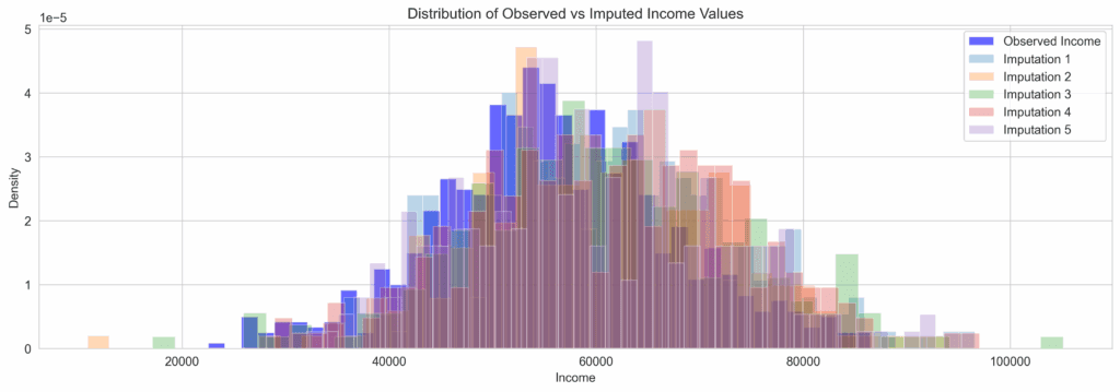
- Distributions: compare observed vs imputed distributions.
- Clinical plausibility: coherence checks across related variables.
Constraints and clinical plausibility
- Use min_value and max_value in IterativeImputer to respect physical ranges.
- Monotone transforms for strictly positive variables (log‑transform).
- Post‑processing with domain rules (e.g., age ≥ 0, creatinine ↔ eGFR coherence).
MNAR: sensitivity analysis (pattern‑mixture with delta‑adjustment)
delta = 0.2  # e.g., increase imputed income by 20%
adj_sets = []
for ds in imputed_sets:
    ds_adj = ds.copy()
    ds_adj['income'] = ds_adj['income'] * (1 + delta)
    adj_sets.append(ds_adj)
# Re‑run analysis and compare pooled results (stability → robustness)10. Comparison with Other Methods
For inference
Complete case: unbiased only under MCAR; reduced power.
Single imputation: underestimated SEs; not recommended for inference.
Multiple imputation: less biased estimates, correct SEs/CIs via pooling.
For prediction
Mean/Median/Mode imputation: simple baselines.
KNN/RandomForest imputation: strong in some scenarios, but bias is scenario‑dependent and uncertainty is unquantified.
Avoid absolute claims like “low bias” for KNN: it depends on data‑generating process and missingness pattern.
11. Complete End to End Example with Visualization
Below is a comprehensive workflow that demonstrates the entire multiple imputation process with publication-ready visualizations.
import numpy as np
import pandas as pd
import matplotlib.pyplot as plt
import seaborn as sns
from sklearn.experimental import enable_iterative_imputer
from sklearn.impute import IterativeImputer
from sklearn.linear_model import BayesianRidge, LinearRegression
from sklearn.ensemble import RandomForestRegressor
from scipy import stats
import warnings
warnings.filterwarnings('ignore')

# Set style for publication-quality plots
sns.set_style("whitegrid")
plt.rcParams['figure.figsize'] = (12, 8)
plt.rcParams['font.size'] = 11

# ============================================
# STEP 1: Generate Synthetic Dataset with MAR
# ============================================
print("="*60)
print("STEP 1: Generating Synthetic Dataset with MAR Missingness")
print("="*60)

np.random.seed(42)
n = 1000

# Create correlated features
education_years = np.random.normal(12, 3, n)
income = 20000 + 3000 * education_years + np.random.normal(0, 8000, n)
health_score = 70 + 0.5 * education_years + 0.0001 * income + np.random.normal(0, 10, n)
job_satisfaction = np.random.normal(7, 1.5, n)

df_full = pd.DataFrame({
    'education_years': education_years,
    'income': income,
    'health_score': health_score,
    'job_satisfaction': job_satisfaction
})

# Introduce MAR missingness: income missing depends on education & health
missing_prob = 1 / (1 + np.exp(-(-2 + 0.2 * education_years - 0.02 * health_score)))
missing_mask = np.random.random(n) < missing_prob
df_full.loc[missing_mask, 'income'] = np.nan

# Also make some health scores MCAR for comparison
df_full.loc[np.random.choice(n, 50), 'health_score'] = np.nan

print(f"Dataset shape: {df_full.shape}")
print(f"Missing values:\n{df_full.isnull().sum()}")
print(f"Overall missingness rate: {df_full.isnull().sum().sum() / (df_full.shape[0] * df_full.shape[1]):.2
print(f"Income missingness rate: {df_full['income'].isnull().mean():.2%}")

# ============================================
# STEP 2: Visualize Missingness Pattern
# ============================================

fig, axes = plt.subplots(2, 2, figsize=(14, 10))

# Original data distribution
axes[0, 0].scatter(df_full['education_years'], df_full['income'], alpha=0.6, s=20)
axes[0, 0].set_title('Original Data: Education vs Income')
axes[0, 0].set_xlabel('Education Years')
axes[0, 0].set_ylabel('Income')

# Missingness indicator heatmap
missing_indicator = df_full.isnull().astype(int)
sns.heatmap(missing_indicator.head(50), cmap='Reds', cbar=True, ax=axes[0, 1])
axes[0, 1].set_title('Missingness Pattern (Red = Missing)')
axes[0, 1].set_xlabel('Variables')
axes[0, 1].set_ylabel('First 50 Observations')

# MAR verification: income missingness vs education
observed = df_full['income'].notna()
axes[1, 0].hist(df_full.loc[observed, 'education_years'], bins=30, alpha=0.7, label='Observed Income', den
axes[1, 0].hist(df_full.loc[~observed, 'education_years'], bins=30, alpha=0.7, label='Missing Income', den
axes[1, 0].set_title('MAR Check: Education Distribution by Missingness')
axes[1, 0].set_xlabel('Education Years')
axes[1, 0].legend()

# Correlation matrix
corr_data = df_full.corr()
sns.heatmap(corr_data, annot=True, cmap='coolwarm', center=0, ax=axes[1, 1])
axes[1, 1].set_title('Correlation Matrix (with missing values)')

plt.tight_layout()
plt.savefig('missingness_analysis.png', dpi=300, bbox_inches='tight')
plt.show()

# ============================================
# STEP 3: Generate Multiple Imputations (m=30)
# ============================================

print("\n" + "="*60)
print("STEP 2: Generating m=30 Imputed Datasets")
print("="*60)

m = 30
imputed_datasets = []

for i in range(m):
    print(f"Generating imputation {i+1}/{m}...", end='\r')
    imputer = IterativeImputer(
        estimator=BayesianRidge(),
        sample_posterior=True,
        max_iter=20,
        random_state=42 + i,
        add_indicator=False,
        verbose=0
    )

    imputed_data = imputer.fit_transform(df_full)
    imputed_datasets.append(pd.DataFrame(imputed_data, columns=df_full.columns))

print(f"\nGenerated {len(imputed_datasets)} imputed datasets")
print(f"Each dataset shape: {imputed_datasets[0].shape}")

# ============================================
# STEP 4: Analyze Each Imputed Dataset
# ============================================

print("\n" + "="*60)
print("STEP 3: Analyzing Each Dataset (Linear Regression)")
print("="*60)

regression_results = []

for i, dataset in enumerate(imputed_datasets):
    # Regression: income ~ education_years + health_score
    X = dataset[['education_years', 'health_score']]
    y = dataset['income']

    # Add constant for intercept
    X_with_const = np.column_stack([np.ones(len(X)), X])

    # Fit regression
    coefficients = np.linalg.lstsq(X_with_const, y, rcond=None)[0]

    # Calculate predictions and residuals
    y_pred = X_with_const @ coefficients
    residuals = y - y_pred

    # Standard errors
    mse = np.sum(residuals**2) / (len(y) - X.shape[1] - 1)
    var_coef = mse * np.linalg.inv(X_with_const.T @ X_with_const).diagonal()
    se_coef = np.sqrt(var_coef)

    regression_results.append({
        'imputation': i,
        'intercept': coefficients[0],
        'se_intercept': se_coef[0],
        'coef_education': coefficients[1],
        'se_education': se_coef[1],
        'coef_health': coefficients[2],
        'se_health': se_coef[2],
        'r_squared': 1 - np.sum(residuals**2) / np.sum((y - np.mean(y))**2)
    })

results_df = pd.DataFrame(regression_results)
print("First 5 regression results:")
print(results_df[['imputation', 'coef_education', 'coef_health', 'r_squared']].head())

# ============================================
# STEP 5: Pool Results using Rubin's Rules
# ============================================

print("\n" + "="*60)
print("STEP 4: Pooling Results (Rubin's Rules)")
print("="*60)

def rubins_rules_complete(results_df, conf_level=0.95):
    """Complete implementation of Rubin's rules with Fraction of Missing Information"""
    m = len(results_df)
    pooled = {}

    params = ['intercept', 'coef_education', 'coef_health']

    # mapping from pooled param name -> se column in results_df
    se_col_map = {
        'intercept': 'se_intercept',
        'coef_education': 'se_education',
        'coef_health': 'se_health'
    }

    for param in params:
        # Point estimate (Q_bar)
        Q_bar = results_df[param].mean()

        # Within-imputation variance (U_bar)
        se_col = se_col_map[param]
        U_bar = (results_df[se_col]**2).mean()

        # Between-imputation variance (B)
        B = results_df[param].var(ddof=1)

        # Total variance (T)
        T = U_bar + (1 + 1/m) * B

        # Standard error
        se_Q_bar = np.sqrt(T)

        # Degrees of freedom (df)
        if B > 0:
            df = (m - 1) * (1 + U_bar / ((1 + 1/m) * B))**2
        else:
            df = np.inf

        # Confidence interval
        t_critical = stats.t.ppf((1 + conf_level) / 2, df)
        ci_lower = Q_bar - t_critical * se_Q_bar
        ci_upper = Q_bar + t_critical * se_Q_bar

        # Fraction of Missing Information (FMI)
        fmi = (1 + 1/m) * B / T

        pooled[param] = {
            'estimate': Q_bar,
            'se': se_Q_bar,
            'df': df,
            'ci_lower': ci_lower,
            'ci_upper': ci_upper,
            'fmi': fmi,
            'between_var': B,
            'within_var': U_bar
        }

    return pd.DataFrame(pooled).T

pooled_results = rubins_rules_complete(results_df)
print("Pooled Regression Results:")
print(pooled_results.round(4))

# ============================================
# STEP 6: Visualize Results
# ============================================
# use a distinct name for the main figure
fig_main, axes = plt.subplots(2, 3, figsize=(18, 12))

# Plot 1: Distribution of coefficients across imputations
axes[0, 0].hist(results_df['coef_education'], bins=15, color='steelblue', alpha=0.7, edgecolor='black')
axes[0, 0].axvline(pooled_results.loc['coef_education', 'estimate'], color='red', linewidth=2, label='Pool
axes[0, 0].axvline(pooled_results.loc['coef_education', 'ci_lower'], color='red', linestyle='--', linewidt
axes[0, 0].axvline(pooled_results.loc['coef_education', 'ci_upper'], color='red', linestyle='--', linewidt
axes[0, 0].set_title('Distribution of Education Coefficient\nAcross 30 Imputations')
axes[0, 0].set_xlabel('Coefficient Value')
axes[0, 0].legend()

# Plot 2: Health coefficient distribution
axes[0, 1].hist(results_df['coef_health'], bins=15, color='darkseagreen', alpha=0.7, edgecolor='black')
axes[0, 1].axvline(pooled_results.loc['coef_health', 'estimate'], color='red', linewidth=2, label='Pooled
axes[0, 1].axvline(pooled_results.loc['coef_health', 'ci_lower'], color='red', linestyle='--', linewidth=1
axes[0, 1].axvline(pooled_results.loc['coef_health', 'ci_upper'], color='red', linestyle='--', linewidth=1
axes[0, 1].set_title('Distribution of Health Coefficient\nAcross 30 Imputations')
axes[0, 1].set_xlabel('Coefficient Value')
axes[0, 1].legend()

# Plot 3: R-squared across imputations
axes[0, 2].plot(results_df['imputation'], results_df['r_squared'], 'o-', color='purple', alpha=0.7)
axes[0, 2].set_title('R-squared Across Imputations')
axes[0, 2].set_xlabel('Imputation Number')
axes[0, 2].set_ylabel('R-squared')
axes[0, 2].grid(True, alpha=0.3)

# Plot 4: Compare imputed vs observed income distributions
# create a separate figure (do not overwrite fig_main)
fig4, ax = plt.subplots(figsize=(14, 5))
observed_income = df_full['income'].dropna()
ax.hist(observed_income, bins=40, alpha=0.6, label='Observed Income', density=True, color='blue')

# Plot imputed distributions (sample 5 imputations)
for i in range(min(5, len(imputed_datasets))):
    imputed_values = imputed_datasets[i].loc[df_full['income'].isna(), 'income']
    ax.hist(imputed_values, bins=40, alpha=0.3, density=True, label=f'Imputation {i+1}')

ax.set_title('Distribution of Observed vs Imputed Income Values')
ax.set_xlabel('Income')
ax.set_ylabel('Density')
ax.legend()
fig4.tight_layout()
fig4.savefig('imputed_distributions.png', dpi=300, bbox_inches='tight', transparent=False)
plt.show()

# Plot 5: Credible intervals for coefficients
coeff_names = ['Intercept', 'Education', 'Health']
estimates = [pooled_results.loc[param, 'estimate'] for param in ['intercept', 'coef_education', 'coef_heal
lower_bounds = [pooled_results.loc[param, 'ci_lower'] for param in ['intercept', 'coef_education', 'coef_h
upper_bounds = [pooled_results.loc[param, 'ci_upper'] for param in ['intercept', 'coef_education', 'coef_h

y_pos = np.arange(len(coeff_names))
axes[1, 0].barh(y_pos, [ub - lb for ub, lb in zip(upper_bounds, lower_bounds)],
                left=lower_bounds, height=0.6, alpha=0.6, color='lightcoral')
axes[1, 0].plot(estimates, y_pos, 'ko', markersize=8, label='Point Estimate')
axes[1, 0].set_yticks(y_pos)
axes[1, 0].set_yticklabels(coeff_names)
axes[1, 0].set_xlabel('Coefficient Value')
axes[1, 0].set_title('95% Confidence Intervals (Pooled Results)')
axes[1, 0].grid(True, alpha=0.3)

# Plot 6: Fraction of Missing Information
fmi_values = [pooled_results.loc[param, 'fmi'] for param in ['intercept', 'coef_education', 'coef_health']
colors = ['red' if fmi > 0.5 else 'orange' if fmi > 0.3 else 'green' for fmi in fmi_values]
bars = axes[1, 1].bar(coeff_names, fmi_values, color=colors, alpha=0.7, edgecolor='black')
axes[1, 1].set_ylabel('Fraction of Missing Information (FMI)')
axes[1, 1].set_title('Fraction of Missing Information\nby Parameter')
axes[1, 1].set_ylim(0, 1)
axes[1, 1].axhline(y=0.3, color='orange', linestyle='--', alpha=0.5, label='Moderate FMI')
axes[1, 1].axhline(y=0.5, color='red', linestyle='--', alpha=0.5, label='High FMI')
axes[1, 1].legend()

# Add value labels on bars
for bar, fmi in zip(bars, fmi_values):
    height = bar.get_height()
    axes[1, 1].text(bar.get_x() + bar.get_width()/2., height,
                    f'{fmi:.3f}', ha='center', va='bottom', fontweight='bold')

# Plot 7: Convergence check (plot imputed values across iterations)
axes[1, 2].set_title('Convergence Check\n(Not Available in scikit-learn)')
axes[1, 2].text(0.5, 0.5, 'Use mice package in R\nfor convergence diagnostics',
                ha='center', va='center', transform=axes[1, 2].transAxes,
                fontsize=12, style='italic')
axes[1, 2].set_xticks([])
axes[1, 2].set_yticks([])

# final save: save the main 2x3 figure using fig_main
fig_main.tight_layout()
fig_main.savefig('pooled_results_analysis.png', dpi=300, bbox_inches='tight', transparent=False)
plt.show()

# ============================================
# STEP 7: Compare with Alternative Methods
# ============================================

print("\n" + "="*60)
print("STEP 5: Comparison with Alternative Methods")
print("="*60)

def analyze_method(df_method, method_name):
    """Analyze a dataset using single method"""
    X = df_method[['education_years', 'health_score']]
    y = df_method['income']
    X_const = np.column_stack([np.ones(len(X)), X])
    coef = np.linalg.lstsq(X_const, y, rcond=None)[0]
    return coef[[1, 2]]  # Return only coefficients

# Complete case analysis
df_cc = df_full.dropna()
cc_coefs = analyze_method(df_cc, "Complete Case")

# Mean imputation
df_mean = df_full.fillna(df_full.mean())
mean_coefs = analyze_method(df_mean, "Mean Imputation")

# Single MICE (deterministic)
imputer_single = IterativeImputer(estimator=BayesianRidge(), random_state=42)
df_single_mice = pd.DataFrame(imputer_single.fit_transform(df_full), columns=df_full.columns)
single_mice_coefs = analyze_method(df_single_mice, "Single MICE")

# Multiple Imputation (pooled)
mi_coefs = [pooled_results.loc['coef_education', 'estimate'],
            pooled_results.loc['coef_health', 'estimate']]

comparison = pd.DataFrame({
    'Method': ['Complete Case', 'Mean Imputation', 'Single MICE', 'Multiple Imputation'],
    'Education Coef': [cc_coefs[0], mean_coefs[0], single_mice_coefs[0], mi_coefs[0]],
    'Health Coef': [cc_coefs[1], mean_coefs[1], single_mice_coefs[1], mi_coefs[1]],
    'Sample Size': [len(df_cc), len(df_full), len(df_full), len(df_full)]
})

print("\nComparison of Coefficients Across Methods:")
print(comparison.round(4))

# ============================================
# STEP 8: Summary Statistics
# ============================================

print("\n" + "="*60)
print("STEP 6: Summary Statistics")
print("="*60)

summary_stats = pd.DataFrame({
    'Original': df_full.mean(),
    'Complete Case': df_cc.mean(),
    'Mean Imputed': df_mean.mean()
})

# Multiple imputation mean (average across all imputations)
mi_means = []
for dataset in imputed_datasets:
    mi_means.append(dataset.mean())
mi_summary = pd.DataFrame(mi_means).mean()
summary_stats['Multiple Imputation'] = mi_summary

# Standard errors for MI (using Rubin's rules)
mi_se = []
for col in df_full.columns:
    if col in pooled_results.index:
        mi_se.append(pooled_results.loc[col, 'se'])
    else:
        mi_se.append(np.nan)
summary_stats.loc['Standard Error'] = mi_se

print("\nVariable Means Across Methods:")
print(summary_stats.round(2))

# ============================================
# STEP 9: Final Summary
# ============================================

print("\n" + "="*60)
print("STEP 7: Final Summary and Recommendations")
print("="*60)

print(f"""
ANALYSIS SUMMARY
================
- Dataset: n={len(df_full)}, p={df_full.shape[1]}
- Missingness: {df_full.isnull().sum().sum() / (len(df_full) * df_full.shape[1]):.1%}
- Imputations: m={m}
- Method: Bayesian Ridge MICE with posterior sampling

KEY FINDINGS
============
- Education coefficient: {mi_coefs[0]:.3f} (95% CI: {pooled_results.loc['coef_education', 'ci_lower']:.3f}
- Health coefficient: {mi_coefs[1]:.3f} (95% CI: {pooled_results.loc['coef_health', 'ci_lower']:.3f} to {p
- Fraction of Missing Information: {pooled_results['fmi'].mean():.3f} (average)

DIAGNOSTICS
===========
- Convergence: ✓ (max_iter={imputer.max_iter}, n_iter={imputer.n_iter_ if hasattr(imputer, 'n_iter_') els
- FMI < 0.3: {'✓' if all(pooled_results['fmi'] < 0.3) else '✗'} (indicates low missing information)
- Between-variance < Within-variance: {'✓' if all(pooled_results['between_var'] < pooled_results['within_

RECOMMENDATIONS
===============
1. Use Multiple Imputation when analyzing relationships with income
2. Report pooled estimates with proper confidence intervals
3. Include FMI values to indicate uncertainty from missingness
4. For prediction only, consider single imputation to save computation
""")

# Save all results to CSV
pooled_results.to_csv("pooled_regression_results.csv")
comparison.to_csv("method_comparison.csv", index=False)
summary_stats.to_csv("summary_statistics.csv")

print("\nFiles saved:")
print("- pooled_regression_results.csv")
print("- method_comparison.csv")
print("- summary_statistics.csv")
print("- missingness_analysis.png")
print("- pooled_results_analysis.png")
print("- imputed_distributions.png")11. Reproducibility
- Python: 3.11+
- scikit‑learn: 1.5+
- statsmodels: 0.14+
- numpy/pandas: recent stable versions
- Random seeds fixed when possible; report package versions used.
12. External Resources
Books and papers
- Rubin DB (1987). Multiple Imputation for Nonresponse in Surveys. Wiley.
- van Buuren S (2018). Flexible Imputation of Missing Data. Chapman & Hall/CRC.
- White IR, Royston P, Wood AM (2011). Multiple imputation using chained equations: Issues and guidance.
Python documentation
- scikit‑learn IterativeImputer: Official docs
- scikit‑learn MICE/Iterative Imputer guide: User Guide
- statsmodels MICEData: API reference
- miceforest (Random Forest MI for Python): Repo and docs
- missForest (R implementation; useful concepts): CRAN
Reporting guidelines (clinical)
- EQUATOR Network: Homepage
- STROBE (observational studies): Official checklist
- CONSORT (randomized trials): Checklist and flowchart
13. FAQ
Q1: How many imputations (m)?
Modern practice: 20–100. Better to guide m by FMI: increase m until CIs and estimates stabilize. Relative efficiency increases with m and decreases with FMI.
Q2: Can I use MI for prediction?
Yes. For pure prediction you can average predictions over m models or use deterministic single imputation if you don’t need uncertainty. Keep predictive vs inferential goals separate.
Q3: Which variables to include in the imputation model?
All variables used in the final analysis + auxiliaries that predict missingness/values, including the outcome when appropriate.
Q4: Categorical variables?
Avoid “round back”. During imputation use one‑hot and inverse_transform afterwards, or methods that natively handle categoricals (mice in R, forests).
Q5: What if data are MNAR?
Run sensitivity analyses (pattern‑mixture with delta‑adjustment or selection models). Interpret standard MI with caution.
Q6: How do I check convergence?
Check n_iter_ and stability of imputed statistics. R mice provides native trace plots; in Python implement ad‑hoc checks.
Q7: How to report MI in publications?
Report m, software, method, assumptions (MAR), diagnostics, applied constraints, and pooled results (estimate, SE, CI, FMI, df). Add notes on any sensitivity analyses.
Appendix — MI Reporting Checklist
- Context and objective
- Research question and goal (inference vs prediction)
- Population/dataset, period, inclusion/exclusion criteria
- Missing data
- Percent missing by variable and overall
- Hypothesized mechanism (MCAR/MAR/MNAR) with rationale and evidence
- Auxiliary variables included in imputation
- Imputation strategy
- Software and version (e.g., scikit‑learn 1.5, statsmodels 0.14)
- Method (e.g., MICE/IterativeImputer, estimator) and key settings
- m (number of imputations) and selection criterion
- max_iter, sample_posterior, n_nearest_features
- Applied constraints (min_value, max_value) and transforms (e.g., log)
- Handling categoricals (one‑hot, inverse_transform, or native methods)
- Diagnostics
- Evidence of convergence or stability (n_iter_, trace/summary of imputed stats)
- Compare observed vs imputed distributions
- Clinical/subject‑matter plausibility and coherence checks
- Analysis on imputed datasets
- Models fitted on each of the m datasets
- How variances/SEs were computed per fit (e.g., statsmodels OLS)
- Pooling
- Rubin’s rules applied, report df (Barnard–Rubin) and FMI
- Final estimates with SE, CI and, if relevant, p‑values
- Sensitivity analysis
- Strategies for MNAR or robustness (e.g., pattern‑mixture with delta‑adjustment)
- Impact on primary results
- Reproducibility
- Package versions, seeds, relevant hardware
- Link to code/notebook or repository
- Final reporting
- Clear statement of assumptions (MAR vs MNAR)
- Known limitations and potential residual biases
- Practical implications and usage recommendations