
Normality testing is still routine in medical research. The familiar rule, “Shapiro–Wilk significant, therefore Mann–Whitney,” is not a sound decision tree. A practical, reproducible guide for clinical researchers.
Author: Michele D. Pierri
Category: Statistics · Data Analysis · Clinical Research
Reading time: approximately 15 minutes
Last updated: November 2026
The question almost every clinical researcher has been asked
Imagine you are comparing postoperative intensive care length of stay between two groups of cardiac surgery patients. You run a Shapiro–Wilk test and it returns p < 0.001. You replace the planned t-test with a Mann–Whitney test, write that “continuous variables were tested for normality,” and move on.
Familiar? It should be. The sentence appears in countless Methods sections, I suspect most of us have written it at least once, and some reviewers explicitly ask for it. But what has the Shapiro–Wilk test actually established? Has it shown that the original analysis would have been invalid? And does Mann–Whitney answer the same question as the t-test?
Usually, no. Testing normality is not forbidden. The problem is letting a preliminary significance test make the methodological decision for us.
In a 2015 commentary in Animal Behaviour, Graeme Ruxton and colleagues took aim at exactly this habit: using a normality test to choose between parametric and non-parametric analyses, a practice they described as inadvisable or, at best, unnecessary [1]. Later methodological work has reinforced the argument and, in places, qualified it [2–8]. What emerges is more demanding than simply dropping a test. Choose the analysis that answers the scientific question. Diagnose the assumptions that matter for that analysis. Then check whether the conclusion survives reasonable alternatives.
This article develops the idea with five original figures, simulated examples and a reproducible Python script. No real patient data are used.
1. What does a normality test actually test?
Shapiro–Wilk tests the null hypothesis that the observations come from a normally distributed population. A significant result is evidence against that model. A nonsignificant one means we have failed to reject normality, which is not the same as having proved it.
Why does that distinction carry so much weight? Because the test responds to two things at once: the shape of the underlying distribution and the number of observations.
A small sample can hide substantial departures from normality. A large one can flag a departure so slight that it has no practical effect on the estimate or inference we actually care about. This is not a peculiarity of Shapiro–Wilk; every hypothesis test behaves this way. Ruxton and colleagues noted that even the better normality tests generally have power below 0.5 with fewer than 50 observations [1]. Shapiro–Wilk can be useful. Its p-value, though, is not a universal certificate of validity for some other analysis [1, 2, 7].
Simulation 1: same population, different sample size
The first figure shows how often Shapiro–Wilk rejects normality in samples drawn from three fixed populations: a genuinely normal distribution, a mildly skewed lognormal and a more strongly skewed lognormal. For each sample size, the Python script generates 500 independent datasets and counts the proportion of tests with p < 0.05.
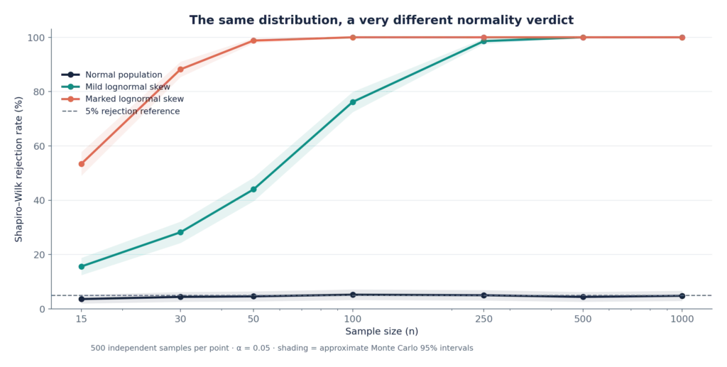
Figure 1. The probability that Shapiro–Wilk rejects normality depends strongly on sample size. Shaded intervals represent approximate Monte Carlo uncertainty, not clinical confidence intervals.
For the mildly skewed population, normality was rejected in 28.2% of samples at n = 30 and in 98.6% at n = 250. The generating distribution never changed. Only the sample size did. With truly normal data, the rejection rate stayed close to the nominal 5%.
These percentages come from our fixed-seed simulation, not from Ruxton’s paper, and re-running the supplied script reproduces them.
Clinical implication: reading p = 0.12 in a study of 25 patients as proof that a variable is normal is a category error. So is reading p < 0.001 in a study of 2,000 patients as proof that a parametric comparison is invalid.
2. A normality test often examines the wrong object
Of everything in this discussion, this is the point I would most like readers to keep.
When we compare sample means or estimate regression coefficients, the quantity whose sampling behavior matters is not necessarily the individual observation. For a sample mean, what counts is the sampling distribution of the mean. In a classical linear model, exact small-sample Gaussian inference concerns the model errors (conditional on the predictors), not the unconditional distribution of the outcome and certainly not the distribution of every predictor.
These are different distributions. So which one was the routine Shapiro–Wilk test looking at? Usually the first, and the least relevant.
Simulation 2: individual values versus sample means
Suppose a biomarker follows an exponential distribution: most values are low, and a minority are much higher. Many of the variables we collect after cardiac surgery, peak lactate or chest drain output in the first 24 hours among them, tend to look like this. The population distribution is clearly right-skewed. We repeatedly draw independent samples and look at their means.
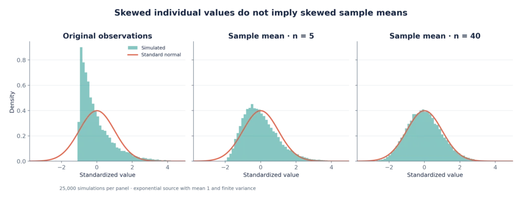
Figure 2. Standardized individual observations remain skewed, while the distribution of means approaches the normal curve as sample size increases. The red line is the standard normal density.
The central limit theorem explains why the distribution of a sample mean often becomes approximately Gaussian as sample size grows, even when individual measurements are not. That is a large part of why many mean-based tests and estimators are robust [3, 4].
There is, however, no magic threshold at n = 30. How quickly the approximation improves depends on skewness, tail behavior, independence, group balance and the existence of a finite variance. Heavy tails, rare extreme values and very unequal groups can all make familiar approximations unreliable.
And the theorem rescues nothing else. Not a poorly defined outcome. Not a biased cohort. Not correlated measurements analyzed as if they were independent.
3. In regression, normality of the outcome is not the standard assumption
Consider a linear regression:
Yi = β0 + β1 Xi + εi.
The conventional Gaussian model specifies the distribution of the error term conditional on the predictors. In general it says nothing about the marginal distribution of Y, or about the distribution of X.
In the next example X is strongly right-skewed, while the errors are generated from a normal distribution. The observed outcome is therefore right-skewed, yet the residuals from the fitted linear model are approximately normal.
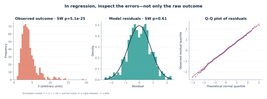
Figure 3. In this simulated regression (n = 600), Shapiro–Wilk applied to the raw outcome gives p = 5.1 × 10⁻²⁵; applied to fitted residuals, p = 0.614. The model errors were generated as Gaussian by design.
A rule that says “test every continuous variable for normality” misses the point in regression, because it checks something other than the model’s central assumptions. Midway and White reviewed regression practice in ecology and biology and found that more than 70% of ecology papers and 90% of biology papers applied normality tests to the raw data rather than to the residuals [6]. To be fair, their simulations found that the mistake cost surprisingly little power, especially in larger samples, and the title of their paper admits as much. A conceptual error and a practical disaster are not the same thing.
Does that make the error harmless? Not quite, because even residual normality is not the whole story. Depending on the inferential procedure, we should also examine functional form, heteroscedasticity, influential observations, independence, clustering and model specification. Normal errors matter for exact classical small-sample inference, but normally distributed residuals do not repair a violation of independence or a misspecified model.
For logistic, Poisson and survival models the standard assumptions are different again, and demanding normally distributed outcome data makes little sense.
4. The deeper problem: the tests may answer different questions
Many textbooks present Student’s t-test and Mann–Whitney as interchangeable ways of comparing two groups: normal observations, use t; otherwise, use Mann–Whitney.
In general, though, the two procedures do not target the same estimand.
- Welch’s t-test targets the difference between population means, and its usual standard error does not require equal population variances.
- The Mann–Whitney U test is rank-based. Its standard null hypothesis is that the two distributions are equal, and its statistic is closely related to the probability that a randomly chosen observation from one group exceeds a randomly chosen observation from the other. It is sensitive to some differences between distributions, but not to every possible difference, and it is not automatically a test of equal medians. Reading it as a median shift requires extra assumptions, such as similarly shaped distributions.
How often have you seen a Mann–Whitney p-value printed next to two medians, as if it had compared them?
Simulation 3: equal means, different distributions
We generated two independent groups of 2,500 observations. Group A follows an exponential distribution with population mean 1. Group B follows a lognormal distribution whose parameters were chosen so that its population mean is also exactly 1. Their shapes and medians differ substantially.
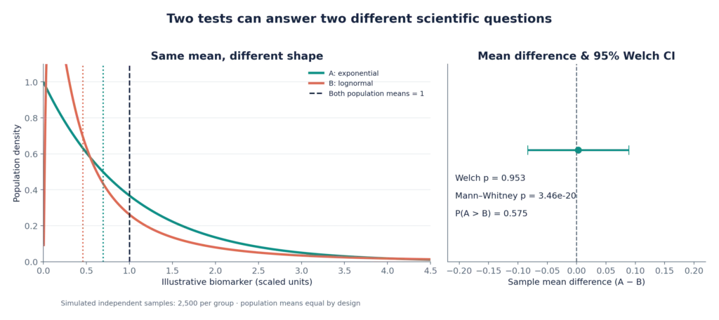
Figure 4. The two generating populations have the same mean by construction. In one reproducible realization, Welch p = 0.953, Mann–Whitney p = 3.46 × 10⁻²⁰. These are not contradictory findings: the procedures target different properties.
In this realization the estimated difference between sample means (A − B) is about 0.003, with a 95% Welch confidence interval of −0.084 to 0.089. The Mann–Whitney result corresponds to an empirical P(A > B) of about 0.575 (there are no ties in these continuous simulated data). Group A produces the larger observation more often, even though both populations share the same mean.
Has Mann–Whitney produced a false positive? No. The two populations really are different; the test has simply picked up a property other than a difference in means. Fagerland described the same interpretive problem in extensive simulation work [5].
So the practical question is not “Which test gives significance?” It is “Which population quantity answers the clinical question?”
Take length of stay. We may care about mean bed-days, for resource planning; about the typical patient’s experience, summarized by the median; about the probability of a prolonged admission; or about time to discharge when death competes with it. Each is a legitimate question, and each calls for a different analysis. In cardiac surgery the last one is far from a technicality. A patient who dies on the third postoperative day has a short ICU stay, and no sensible analysis should let that count as a good outcome.
5. Does this mean the t-test is always robust?
No. Swapping the Shapiro decision tree for “always use Welch” would just be a different oversimplification.
Large, balanced samples and moderately skewed outcomes often allow useful mean-based inference. Small samples, severe skewness, heavy tails, extreme observations and markedly unequal group sizes are another matter. Heteroscedasticity can distort Student’s equal-variance test, and the familiar Welch approximation is not immune to every combination of skewness and imbalance.
De Winter’s 2026 simulation study puts numbers on this. With unequal sample sizes and skewed distributions, Welch’s test produced false-positive rates of roughly 6%, 7.5% and 9% at skewness values of 1, 2 and 3, against a nominal 5% [8]. A permutation-based version of Welch’s test held the nominal rate across the whole simulation design, and the Anderson–Darling test performed well when the real question was whether two distributions differ at all. One simulation study does not crown a universally optimal test, of course. Design, estimand and assumptions still govern the choice.
Depending on the research question, the alternatives include robust standard errors, trimmed-mean procedures, carefully constructed bootstrap intervals, permutation methods, generalized linear models, quantile regression and survival analysis. None of them should be chosen to obtain a convenient p-value. Bootstrap and permutation methods carry assumptions of their own, and naïve resampling is particularly risky with clustering, dependence or nonexchangeable observations.
6. A better workflow for clinical research
Rather than using Shapiro–Wilk as the first branching point, this is the workflow I would follow.
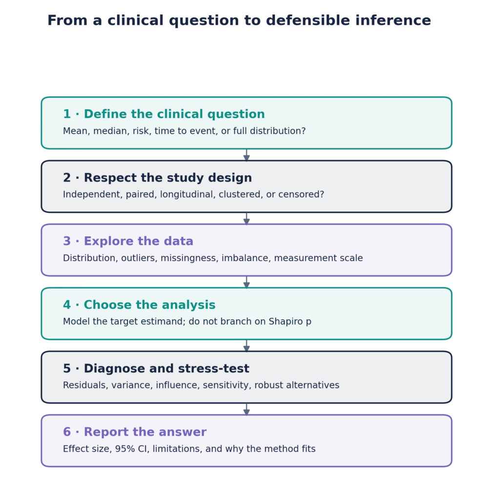
Figure 5. A practical workflow: first define the target of inference, then select and evaluate an appropriate analysis.
What does that look like in practice? The examples below show why the order is more useful than any normality checklist.
| Clinical situation | First question | Reasonable direction |
|---|---|---|
| Two independent groups, continuous outcome, mean is of interest | Are observations independent, and are severe tails or imbalance present? | Mean difference with 95% CI; Welch in suitable settings; robust sensitivity analysis when needed |
| Small study with marked skewness | What feature of the outcome is scientifically important? | Consider robust location estimates, quantile methods, rank methods or carefully justified resampling |
| Repeated postoperative lactate measurements | Is the interest a time trajectory or a single endpoint? | A longitudinal model that accounts for within-patient correlation |
| Length of ICU stay | Is the target mean days, typical stay, or time to discharge? | Define discharge, death, transfer and coding rules; choose a matching outcome model |
| Binary postoperative complication | What is the risk or risk difference? | Binomial/logistic framework; no normality requirement for the binary outcome |
| Prediction model | Are predicted risks calibrated and clinically useful? | Evaluate calibration, discrimination, uncertainty and validation rather than testing the normality of predictors |
This piece complements two earlier guides on this site, Non-Parametric Statistics in Medicine and the Central Limit Theorem. Its emphasis on estimands and interpretation also connects to Effect Size and Calibration of Predictive Risk Models.
Description is not the same as inference
A strongly skewed variable may be best described with the median and interquartile range. That does not oblige the inferential comparison to be a Mann–Whitney test. If the scientific estimand is a mean difference, mean-based inference may still be appropriate under defensible conditions.
The reverse holds as well: reporting a mean and standard deviation does not, by itself, legitimize a t-test. Description tells the reader how the data behave. Inference targets a parameter under a set of assumptions. The two should be consistent, but no single automatic rule chooses both.
7. What should we do when reviewers demand a normality test?
This is a real, practical problem. Anyone who submits to clinical journals will sooner or later meet a reviewer who asks for evidence that normality was assessed, or for a justification of a parametric procedure. The request is entirely reasonable when it really means “show me that you examined the assumptions of your model.” It is much harder to defend when it imposes the algorithm “Shapiro–Wilk, then t or Mann–Whitney.”
A constructive reply makes the inferential target explicit, provides the relevant diagnostics and explains why the primary analysis was chosen. If the journal specifically asks for Shapiro–Wilk, the results can go into the supplementary material as descriptive diagnostics, with their limitations stated. What the normality p-value should not do is decide the primary test after the fact.
A response to the reviewer might read:
We thank the reviewer for raising the importance of checking model assumptions. Our primary estimand was the between-group difference in means; the analysis was therefore selected on that basis rather than by preliminary significance testing for normality. We assessed distributional shape and influential values graphically, evaluated the assumptions relevant to the chosen procedure, and performed an appropriate sensitivity analysis. We have clarified this rationale in the Methods. Where requested, Shapiro–Wilk results are provided in the Supplementary Material, but they were not used as a binary criterion for selecting the primary analysis.
One caveat matters more than the wording. Statements about diagnostic checks or sensitivity analyses belong in the reply only if those procedures were actually performed. And if a check reveals a material failure of the chosen method’s assumptions, the finding has to be dealt with, not waved away with a reference to the central limit theorem.
8. A small methodological shift with large consequences
The traditional sequence is familiar:
Test normality → choose parametric/non-parametric test → report p-value.
A more defensible one is:
Define the clinical question and estimand → select an appropriate model → examine the relevant assumptions → test robustness → report effect size, uncertainty, and limitations.
Is this an argument against diagnostics? Quite the opposite. It is an argument for better diagnostics, done for a reason.
Normality is a mathematical model. It is not a credential that data must earn before they can be analyzed. A significant Shapiro–Wilk result does not automatically invalidate a parametric analysis, and a nonsignificant one does not certify it.
In medical research the deeper responsibility lies elsewhere: making sure that the number we estimate, and the uncertainty we attach to it, actually answer the clinical question.
Reproducibility and figure notes
All five illustrations were produced for this article with Python, NumPy, SciPy and Matplotlib. The script uses a fixed random seed (20261101), simulates no identifiable or real patient data and exports every figure as both transparent PNG and SVG. The complete script, the dependency list and the figures are provided in the accompanying package. All numerical results are illustrative: they are neither empirical clinical findings nor direct reproductions of the simulations in the cited papers.
Download the reproducible Python code: The complete script, dependencies, and instructions are available in the Python source package (ZIP). Readers can use it to reproduce the simulations and regenerate all five figures.
References
- Ruxton GD, Wilkinson DM, Neuhäuser M. Advice on testing the null hypothesis that a sample is drawn from a normal distribution. Animal Behaviour. 2015;107:249–252. doi:10.1016/j.anbehav.2015.07.006.
- Rochon J, Gondan M, Kieser M. To test or not to test: Preliminary assessment of normality when comparing two independent samples. BMC Medical Research Methodology. 2012;12:81. doi:10.1186/1471-2288-12-81.
- Lumley T, Diehr P, Emerson S, Chen L. The importance of the normality assumption in large public health data sets. Annual Review of Public Health. 2002;23:151–169. doi:10.1146/annurev.publhealth.23.100901.140546.
- Schmidt AF, Finan C. Linear regression and the normality assumption. Journal of Clinical Epidemiology. 2018;98:146–151. doi:10.1016/j.jclinepi.2017.12.006.
- Fagerland MW. t-tests, non-parametric tests, and large studies—a paradox of statistical practice? BMC Medical Research Methodology. 2012;12:78. doi:10.1186/1471-2288-12-78.
- Midway S, White JW. Testing for normality in regression models: mistakes abound (but may not matter). Royal Society Open Science. 2025;12(4):241904. doi:10.1098/rsos.241904.
- Gosselin R-D. Testing for normality: a user’s (cautionary) guide. Laboratory Animals. 2024;58(5):433–437. doi:10.1177/00236772241276808.
- de Winter J. Neither the t-test nor Welch’s test: a case for robust alternatives in two-sample comparisons with non-ideal data. Quality & Quantity. 2026;60(5):18673–18697. doi:10.1007/s11135-026-02909-5.