Healthcare informatics and medical data management. Topics include DICOM standards, medical databases, electronic health records, and information systems in clinical practice.
Healthcare systems across the world have invested billions in clinical digitalization. Electronic health records (EHRs), clinical data warehouses, integrated hospital platforms, and now artificial intelligence systems have been introduced under the promise of efficiency, transparency, interoperability, and improved patient outcomes.
Yet, after more than two decades of implementation, the recurring pattern remains strikingly consistent: resistance from clinicians, workflow friction, hidden cognitive overload, interoperability failures, and, in many cases, silent abandonment.
The problem is rarely technological immaturity. Nor is it simply “resistance to change”.
The deeper issue is structural: clinical digitalization often fails because it attempts to impose the logic of information systems onto a domain—medicine—that operates according to fundamentally different epistemological principles.
This is not a story of bad software. It is a story of a category error.
Key takeaways (in 60 seconds)
EHR failures are often modeling failures: clinical work is non-linear, contextual, and narrative.
Digitalization changes visibility and power, so adoption is also a governance problem.
“Interoperability” fails when architectures remain closed and vendor-optimized.
Many systems increase cognitive load by externalizing clerical work to clinicians.
AI helps when it reduces clerical friction and mediates semantics, not when it is layered on top of broken workflows.
1. The Illusion of Rational Digitalization
At the outset, digitalization projects appear rational and unavoidable. They promise:
Standardization
Traceability
Efficiency
Data accessibility
Decision support
From a managerial perspective, these objectives are legitimate. Healthcare is complex, costly, and increasingly accountable. Digital systems promise control over that complexity.
However, what appears rational at the level of governance often becomes frictional at the bedside.
Clinicians experience rigidity where administrators see structure.
They perceive surveillance where policymakers see transparency.
They feel increased workload where vendors promise efficiency.
This divergence is not accidental. It reveals a structural mismatch between two different ways of organizing reality.
2. Data Are Not Neutral: Visibility, Power, and Ownership
One of the least discussed dimensions of digitalization is that clinical data are not merely informational assets. They are also instruments of power.
When data become universally visible:
Clinical decisions become retrospectively examinable.
Performance becomes measurable.
Activity becomes comparable.
Digitalization modifies the balance of visibility within institutions.
Questions inevitably arise:
Who can access my clinical data?
Why can others audit my activity while I cannot audit theirs?
Is this system designed to support care—or to monitor me?
These are not irrational fears. They reflect a shift in governance architecture.
Digital systems do not simply store information. They redistribute authority.
Any digitalization project that ignores this political dimension is likely to encounter resistance—not because clinicians oppose technology, but because clinicians understand its institutional implications.
3. The Ontological Error: Treating Patients as Inventory
Software engineering thrives on structured entities:
Defined states
Clear transitions
Deterministic workflows
Stable categories
This logic works remarkably well in administrative domains. Billing, scheduling, inventory management, procurement—these processes are structured, rule-based, and relatively stable.
Clinical medicine is not.
The patient is not a static entity with predefined states. The patient is a dynamic, context-dependent system characterized by uncertainty, incomplete information, evolving trajectories, and narrative complexity.
When software systems model patients as if they were items in a warehouse—admitted, processed, discharged—they inevitably simplify the ontological richness of clinical reality.
This explains a persistent observation: administrative software often works better in hospitals than clinical software.
Administration resembles structured logistics.
Clinical care resembles complex adaptive reasoning.
The failure lies not in programming skill, but in modeling assumptions.
4. The Semantic Problem: Medicine Is Narrative
Medical language is inherently variable.
Consider a simple postoperative complication:
“FA in POD2”
“Episode of paroxysmal atrial fibrillation occurring on postoperative day two”
Both refer to the same phenomenon. Yet clinical expression varies according to habit, context, training, and communicative intent.
Information systems, however, require:
Stable ontologies
Consistent syntax
Standardized coding
Structured data fields
The attempt to compress medical narrative into fixed data-entry schemas inevitably generates friction.
Clinicians compensate by:
Using free-text fields
Entering partial information
Circumventing rigid workflows
Standardization initiatives (ICD, SNOMED, HL7, FHIR) are essential and valuable. Yet they cannot eliminate the fundamental variability of clinical language, because medicine is not merely descriptive. It is interpretive.
Clinical reasoning is contextual, provisional, and narrative-driven. A purely tabular representation cannot fully capture this dimension.
A further complication is that clinical documentation is not only “data”. It is also a medico-legal artifact and a medium of human-to-human communication. Any system that treats notes as mere structured fields will collide with this reality.
5. Cognitive Load and the Hidden Cost of Rigid Systems
Instead of reducing workload, poorly designed systems increase task fragmentation and mental switching.
The result is not only frustration, but measurable cognitive burden. Documentation time expands. Direct patient interaction contracts.
What is rarely measured in digitalization projects is the cognitive cost per clinical action.
Systems are evaluated on deployment success (“go-live”), not on net cognitive efficiency.
When a digital platform adds friction without reducing risk or saving time, clinicians do not reject technology. Clinicians reject inefficiency.
6. Interoperability: The Persistent Illusion
Another recurring failure lies in integration.
Healthcare institutions often deploy multiple systems:
EHR
Laboratory software
Imaging platforms
Administrative modules
Pharmacy systems
In theory, interoperability standards exist. In practice, integration remains partial, fragile, or vendor-dependent.
Data silos persist.
Interfaces are brittle.
APIs are limited.
As a result, clinicians must navigate multiple platforms, duplicating entries and reconciling inconsistencies.
Fragmented architectures generate friction not because integration is technically impossible, but because systems are often built as closed environments optimized for internal coherence rather than modular interoperability.
Without architectural openness, digital ecosystems become digital labyrinths.
A non-technical driver matters here: procurement and incentives. When purchasing decisions reward feature checklists over usability, and lock-in over openness, architectures predictably become closed and brittle.
7. Why Artificial Intelligence Will Not Magically Fix This
The current wave of artificial intelligence in healthcare promises to solve many of these problems.
However, AI is unlikely to correct structural dysfunctions on its own. It will not, by default:
Fix flawed governance structures
Resolve institutional distrust
Repair closed architectures
Eliminate incentive misalignment
Transform rigid workflows into adaptive ones
If deployed on top of structurally misaligned systems, AI risks amplifying existing dysfunctions.
Adding prediction to chaos does not generate coherence.
So where can AI actually help?
8. Where AI Can Actually Help
Despite these limitations, AI does offer meaningful opportunities—if used appropriately.
1. Semantic Mediation
Large language models and NLP systems can translate narrative text into structured representations, reducing the tension between clinical variability and system rigidity.
They can:
Normalize expressions
Map narrative to ontologies
Extract structured variables from free text
This does not eliminate variability, but it can mediate it.
2. Reduction of Clerical Burden
Speech-to-text systems, intelligent pre-filling, and automated documentation support can reduce repetitive administrative tasks.
When AI reduces documentation time rather than increasing it, adoption becomes organic rather than enforced.
3. Adaptive Workflow Orchestration
AI can help design event-driven, non-linear systems that adapt to clinical trajectories rather than forcing clinicians into rigid sequences.
Such systems must remain clinician-in-the-loop, transparent, and auditable.
AI’s value lies not in replacing reasoning, but in absorbing clerical friction.
9. A Minimal Framework for Non-Failing Digital Systems
If digitalization is to succeed, certain structural principles must guide implementation:
Workflow-first design Systems must model real clinical processes before enforcing data structures.
Semantic flexibility with structured back-end mapping Allow narrative input, then translate into structured data through mediation layers.
Measurement of cognitive cost Evaluate systems based on net reduction of clinician time and cognitive burden.
True interoperability Modular architectures, open APIs, and standardized exchange protocols.
Transparent data governance Clarify access rights, audit structures, and visibility symmetry.
Clinician-centered evaluation metrics Success must be measured in time saved, errors reduced, and communication improved—not merely in deployment completion.
To make this concrete, consider a common clinical reality: trajectories branch. A postoperative course can shift quickly from “stable recovery” to “arrhythmia”, “bleeding”, “infection”, “AKI”, or “delirium”, each altering priorities, documentation needs, and team communication. A linear software funnel will always feel wrong against this event-driven logic.
Conclusion: Digitalization Must Adapt to Medicine
Clinical digitalization fails when it attempts to constrain medicine within the deterministic logic of software architecture.
It succeeds only when digital systems acknowledge that medicine is:
Dynamic
Narrative
Uncertain
Context-dependent
Relational
The patient is not an inventory unit.
Clinical reasoning is not a linear transaction.
Healthcare is not a warehouse workflow.
Artificial intelligence may become a powerful mediator between structured systems and narrative medicine—but only if we first correct the structural mismatch at the heart of digital healthcare.
Technology must adapt to clinical epistemology—not the other way around.
FAQ
Isn’t clinician resistance the real problem?
Often, “resistance” is a signal of design debt: misfit between tools and real work, plus legitimate concerns about governance and accountability.
Do standards like FHIR solve interoperability?
Standards help, but interoperability also depends on incentives and architecture. Closed systems can “support standards” and still prevent meaningful modular integration.
Can AI reduce burnout?
Yes, if it removes clerical burden and improves navigation of narrative data. No, if it adds alerts, extra steps, or opaque recommendations to already fragile workflows.
Understanding DICOM Coordinate Systems and Image Orientation: Why Your 3D Volume Looks Upside Down
1. Introduction — Why Orientation Matters
Have you ever opened a medical image and found the anatomy upside down or mirrored?
It’s not your viewer’s fault — it’s about geometry.
DICOM files contain not only pixels, but also the mathematical information that tells a viewer where those pixels belong in the patient’s body.
This information — stored in a few special orientation tags — determines whether your 3D reconstruction looks anatomically correct or completely inverted.
In this article, we’ll explore:
how DICOM defines spatial orientation,
what its key tags actually mean,
and how to verify them in Python.
By the end, you’ll understand why one missing minus sign can literally turn a patient upside down.
2. From Pixels to Space — How Medical Images Have Coordinates
But in medicine, every pixel must correspond to a real point in space, measured in millimeters.
To achieve this, DICOM defines a patient-based coordinate system, called LPS:
L (Left) → x-axis positive toward the patient’s left
P (Posterior) → y-axis positive toward the back
S (Superior) → z-axis positive toward the head
So, instead of just rows and columns, every DICOM slice is a plane positioned in 3D, with its own origin, orientation, and scale.
Some research formats, such as NIfTI, use a different convention called RAS (Right–Anterior–Superior), where the X and Y axes are mirrored relative to DICOM’s LPS system. For clinical DICOM images, however, all coordinates and orientation vectors are defined in the LPS frame, the only one used by PACS viewers and DICOM software.
3. DICOM Tags: How Geometry Is Stored
Every piece of information in a DICOM file is stored as a data element, identified by a tag.
Each data element has four key components:
Field
Meaning
Example
Tag
4-byte identifier (Group,Element) in hex
(0020,0037)
VR (Value Representation)
Data type (e.g., DS = Decimal String)
DS
VM (Value Multiplicity)
How many values (1, 2, 3, 6, …)
6
Value
Actual data stored as text or binary
"1\\0\\0\\0\\-1\\0"
Together, these fields describe everything from patient name to scanner position — but for orientation, three particular tags define where and how each image plane exists in space.
4. The Geometry Trio: IPP, IOP, and PS
These three tags are the geometric foundation of every DICOM image:
Tag
Name
VR
VM
Purpose
Example
(0020,0032)
ImagePositionPatient (IPP)
DS
3
3D coordinates (x, y, z) of the top-left pixel center (mm). Defines where the plane is.
"-121.7\\-23.7\\766.7"
(0020,0037)
ImageOrientationPatient (IOP)
DS
6
Two unit vectors describing row and column directions in patient coordinates. Defines how the plane is oriented.
"1\\0\\0\\0\\-1\\0"
(0028,0030)
PixelSpacing (PS)
DS
2
Physical distance (mm) between pixel centers along rows and columns. Defines scale.
"0.625\\0.625"
All coordinates are expressed in millimeters in the LPS frame.
5. How These Tags Define an Image Plane
Each DICOM image is not just a 2D grid of pixels — it’s a plane positioned in the 3D coordinate system of the patient.
To understand where each pixel lies in space, DICOM combines three pieces of information:
ImagePositionPatient (IPP) → the 3D coordinates of the origin (the center of the top-left pixel).
ImageOrientationPatient (IOP) → two unit vectors defining the row and column directions of the image plane.
PixelSpacing (PS) → the physical distance between adjacent pixels, measured in millimeters.
Together, they define a simple but powerful equation that maps pixel indices (i, j) to their physical location (x, y, z) in the patient’s coordinate system (LPS).
The DICOM Spatial Mapping Formula
According to the DICOM standard (Part 3, Section C.7.6.2.1-1):
P(i,j) = IPP + j · PS[1] · row + i · PS[0] · col
where:
Symbol
Meaning
P(i, j)
3D coordinates (x, y, z) of pixel (i, j) in the patient’s space
IPP
ImagePositionPatient — origin of the image plane (mm)
PS[0]
PixelSpacing for rows (row spacing). It scales the column direction (col).
PS[1]
PixelSpacing for columns (column spacing). It scales the row direction (row).
row
first three values of ImageOrientationPatient (direction cosines of image rows)
col
last three values of ImageOrientationPatient (direction cosines of image columns)
i, j
row and column indices, starting from (0,0) in the top-left corner
Intuitive interpretation
Moving by +1 column (increasing j) shifts you along the row direction (row × PS[1] mm).
Moving by +1 row (increasing i) shifts you along the column direction (col × PS[0] mm).
The origin (0,0) is at the top-left pixel center, whose absolute coordinates are given by IPP.
The plane normal — the direction in which slices are stacked to form a 3D volume — is defined by the cross product:
normal = row × col
Practical insight
This simple affine relationship is what allows 3D reconstruction software (like 3D Slicer, OsiriX, or Weasis) to rebuild a consistent volume.
However, if the normal vector points in the wrong direction (for example, due to swapped axes or inconsistent slice order), the resulting volume will appear flipped — even though all the pixel data are numerically correct.
6. Example: Reading and Interpreting Real Tag Values
Let’s look at a real-world example taken from an actual DICOM header:
This equation allows you to locate any pixel in absolute patient coordinates (LPS).
Step 4 – Analyze the slice orientation
Because the normal vector = [0, 0, -1], the Z-axis decreases as slice numbers increase — meaning that, in 3D, the next slice has a smaller Z value.
If your viewer assumes slices increase along +Z (superior direction), the reconstructed volume will appear upside down.
That’s why understanding the relationship between IOP, IPP, and slice order is essential for correct 3D visualization.
Summary
Concept
Defined by
Direction
Typical interpretation
Origin
ImagePositionPatient
(0,0) pixel center
3D anchor point of slice
Row direction
IOP[0:3]
+X (Left)
Horizontal axis on image
Column direction
IOP[3:6]
±Y (Posterior or Anterior, depending on IOP)
Vertical axis on image
Spacing
PixelSpacing
PS[0] rows → along col • PS[1] cols → along row
Physical scale
Normal
row × col
+Z or –Z (depends on orientation)
Slice stacking direction
In short, each DICOM slice is a mathematically defined plane in the patient’s body.
By combining ImagePositionPatient, ImageOrientationPatient, and PixelSpacing, you can reconstruct where every pixel lies in millimeter-accurate space — and explain exactly why a 3D volume looks “flipped” when these relationships are misunderstood.
7. Python Example — Read, Analyze, and Validate Orientation
The following script extracts and interprets the geometry of your DICOM files:
import numpy as np, pydicomfrom glob import globdefparse_floats(v): s =str(v).replace(',', '\\\\')return np.array([float(x) for x in s.split('\\\\') if x], dtype=float)defread_geometry(ds): ipp = parse_floats(ds.ImagePositionPatient) iop = parse_floats(ds.ImageOrientationPatient) ps = parse_floats(ds.PixelSpacing) row, col = iop[:3], iop[3:] row, col = row/np.linalg.norm(row), col/np.linalg.norm(col) normal = np.cross(row, col)return ipp, row, col, normal, psfiles =sorted(glob("DICOM_STACK/*.dcm"))d1, d2 =map(pydicom.dcmread, files[:2])ipp, row, col, normal, ps = read_geometry(d1)print("IPP:", ipp)print("Row:", row)print("Column:", col)print("Normal:", normal)print("Pixel Spacing:", ps)dz = [np.dot](<http://np.dot>)((read_geometry(d2)[0] - ipp), normal)print("Δ along normal between slice #1 and #2 (mm):", dz)if dz <0:print("Warning: slices are stacked in the opposite direction.")
This lets you verify:
whether row/column vectors are orthogonal;
whether slices increase along the expected direction;
whether the viewer’s 3D reconstruction should appear upright.
8. Common Pitfalls and How to Avoid Them
❌ Assuming file order = anatomical order→ Always check the Z difference between consecutive ImagePositionPatient values.
❌ Mixing coordinate conventions→ DICOM uses LPS; some research tools use RAS (mirrored X/Y).
❌ Ignoring direction cosines→ The slice order alone doesn’t guarantee correct 3D orientation.
❌ Forgetting to normalize vectors→ Precision errors in floating-point values can distort 3D reconstructions.
9. References and further reading
DICOM Standard, Part 3, Section C.7.6.2 — Image Plane Module.[1]
SimpleITK documentation — orientation and DICOM conversion.[2]
MONAI documentation — spatial orientation and metadata.[3]
pydicom documentation — reading and writing headers and orientation tags.[4]
10. Conclusion
The DICOM format encodes geometry with precision — but that precision only helps if you understand it.
By reading and checking ImagePositionPatient, ImageOrientationPatient, and PixelSpacing, you can diagnose most orientation issues before they ruin your 3D visualization.
In medical imaging, orientation is anatomy — and a single misplaced sign can literally turn the patient upside down.
A technical comparison between TCP and UDP protocols implemented in Python: examining performance metrics, security considerations, and practical applications within healthcare systems using FHIR standards for effective data exchange between medical platforms.
Introduction: The Significance of TCP vs UDP
When browsing websites, streaming videos, or making video calls, our data travels across networks using protocols that ensure reliable and efficient delivery. Two transport protocols dominate this landscape: TCP (Transmission Control Protocol) and UDP (User Datagram Protocol).
What fundamental differences exist between these protocols, and how do these differences impact performance in real-world applications?
Table of Contents
In this post, we’ll cover:
The theoretical foundations of TCP and UDP
Their practical differences demonstrated with Python
A hands-on TCP and UDP communication benchmark
Visual analysis of transmission times
An asynchronous implementation using asyncio and aiohttp
Secure Data Transmission in Healthcare IT
Python for Medical Data Transfer
All the code for this project is available on GitHub
TCP vs UDP: Core Concepts Compared
TCP (Transmission Control Protocol)
Connection-oriented: establishes a reliable connection with a three-way handshake, ensuring both parties are ready to communicate before any data transfer begins.
Reliable: guarantees delivery and reorders packets if needed, with mechanisms for acknowledging received data and retransmitting lost packets automatically.
Flow and congestion control: adapts to network conditions by monitoring bandwidth availability and adjusting transmission rates to prevent network congestion and packet loss.
Used for: HTTPS, email, file transfers, SSH, web browsing, database connections, and any application where data integrity is critical.
UDP (User Datagram Protocol)
Connectionless: sends data without setting up a connection, eliminating the overhead associated with connection establishment and termination processes.
Unreliable: no guarantees for delivery or ordering, which means packets may arrive out of sequence, be duplicated, or not arrive at all without automatic notification.
Minimal overhead: faster and lighter due to the absence of connection management, acknowledgments, and retransmission mechanisms found in TCP.
Used for: DNS, video/audio streaming, online gaming, VoIP, live broadcasts, IoT devices, and time-sensitive applications where speed is prioritized over perfect reliability.
Feature
TCP
UDP
Connection
Yes (Handshake)
No
Reliability
Yes
No
Ordering
Guaranteed
Not guaranteed
Speed
Slower
Faster
Use case
File transfer, web
Streaming, real-time gaming
Understanding the socket Module in Python
Python’s socket module provides a low-level networking interface based on the BSD socket API. It supports both TCP (SOCK_STREAM) and UDP (SOCK_DGRAM) protocols, enabling developers to send and receive data across networks.
Key Functions and Concepts
socket.socket(family, type): creates a new socket object for network communication. For our networking purposes, we typically use AF_INET (for IPv4 addressing) and either SOCK_STREAM for TCP connections or SOCK_DGRAM for UDP datagrams, depending on our reliability and performance requirements.
bind((host, port)): assigns a specific network address (combination of IP address and port number) to the socket, effectively reserving that address for the application. This function is primarily used on the server side to establish a known endpoint where clients can connect.
listen(): configures a TCP socket to passively wait for and queue incoming connection requests, transforming it into a listening socket. This method is exclusive to TCP sockets since UDP doesn’t maintain connection state.
accept(): blocks execution and waits for an incoming TCP connection request. When a client connects, it returns a new socket object specifically for that client connection along with the client’s address information.
connect((host, port)): actively initiates a TCP connection from a client socket to a server at the specified address. This triggers the three-way handshake process that establishes a reliable TCP connection.
sendall(data) / sendto(data, addr): transmits the specified data to the connected peer. sendall() is used with TCP connections and ensures all data is sent, while sendto() is used with UDP and requires specifying the destination address with each call.
recv(bufsize) / recvfrom(bufsize): receives incoming data from the peer, with bufsize indicating the maximum amount of data to be received at once. recv() works with established TCP connections, while recvfrom() is used with UDP and additionally returns the sender’s address.
close(): terminates the socket connection and releases the resources associated with it. For TCP sockets, this initiates the connection termination process, while for UDP sockets, it simply frees the socket descriptor.
The socket module operates in a blocking mode by default, which means function calls like recv() or accept() will pause execution until they complete their operation. In our benchmark, we implement threading to enable the server to listen for incoming data without halting the client’s execution flow.
Benchmarking TCP and UDP in Python
Goal
We’ll benchmark the transmission times for 100 simple messages sent between client and server over both TCP and UDP protocols in a local environment.
Setup
Server and client implementations for each protocol
Localhost communication (127.0.0.1)
threading for concurrent server operation
time.time() for precise timing measurements
matplotlib for visualizing performance results
#--------------------# tcp vs udp# di Michele Danilo Pierri# 08/08/2025#--------------------"""What this measures: - UDP: one datagram (request) -> echo (response) per transaction. - TCP: connect -> send -> recv -> close per transaction."""import argparseimport socketimport threadingimport timefrom time import perf_counterimport statistics as statsimport matplotlib.pyplot as plt# ---------------------------# Defaults (tuneable via CLI)# ---------------------------DEFAULT_HOST="127.0.0.1"TCP_PORT=57211UDP_PORT=57212# Small payload accentuates handshake cost for TCPDEFAULT_PAYLOAD=32# bytesREPEAT=400# transactions per protocolPACE=0.001# seconds between transactions to avoid burstsTIMEOUT=2.0# seconds socket timeout# ---------------------------# Servers# ---------------------------deftcp_transaction_server(host:str, port:int):""" Accepts connections in a loop. For each connection: - read exactly one payload (client sends once) - echo it back - close No artificial sleep; this stays 'real'. """with socket.socket(socket.AF_INET, socket.SOCK_STREAM) as s: s.setsockopt(socket.SOL_SOCKET, socket.SO_REUSEADDR, 1) s.bind((host, port)) s.listen(128)whileTrue: conn, _ = s.accept()try:with conn:# Read exactly one message; size unknown to server,# so read once up to some reasonable amount data = conn.recv(65536)if data: conn.sendall(data)exceptConnectionError:continuedefudp_echo_server(host:str, port:int):""" Stateless echo: for each datagram, send it back to sender. """with socket.socket(socket.AF_INET, socket.SOCK_DGRAM) as s: s.setsockopt(socket.SOL_SOCKET, socket.SO_REUSEADDR, 1) s.bind((host, port))whileTrue: data, addr = s.recvfrom(65536)if data: s.sendto(data, addr)# ---------------------------# Clients / Measurements# ---------------------------defmeasure_udp_transactions(host:str, port:int, payload:bytes, n:int):""" For each transaction: - send one datagram - wait for echo - record transaction time (application-level RTT) """ durations = []with socket.socket(socket.AF_INET, socket.SOCK_DGRAM) as c: c.settimeout(TIMEOUT)for _ inrange(n): t0 = perf_counter() c.sendto(payload, (host, port)) data, _ = c.recvfrom(65536) dt = perf_counter() - t0 durations.append(dt) time.sleep(PACE)return durationsdefmeasure_tcp_transactions(host:str, port:int, payload:bytes, n:int):""" For each transaction: - connect() - send payload once - recv echo once - close - record full transaction time (includes handshake) """ durations = []for _ inrange(n): t0 = perf_counter()with socket.socket(socket.AF_INET, socket.SOCK_STREAM) as c: c.settimeout(TIMEOUT)# Optionally disable Nagle to avoid tiny writes coalescing c.setsockopt(socket.IPPROTO_TCP, socket.TCP_NODELAY, 1) c.connect((host, port)) c.sendall(payload)# Expect a single echo; read once is typically enough on localhost/LAN data = c.recv(65536)# Close via context manager dt = perf_counter() - t0 durations.append(dt) time.sleep(PACE)return durations# ---------------------------# Plot helpers# ---------------------------defsummarize(name, arr): mean = stats.mean(arr) med = stats.median(arr) stdev = stats.pstdev(arr)returnf"{name}: mean={mean:.6e}s, median={med:.6e}s, std={stdev:.6e}s, n={len(arr)}"defplot_results(tcp, udp, payload_size):# 1) Boxplot for robust comparison plt.figure(figsize=(9,5)) plt.boxplot([tcp, udp], labels=["TCP per-tx (handshake)", "UDP per-tx"]) plt.title(f"Per-Transaction RTT (echo), payload={payload_size} bytes") plt.ylabel("Seconds") plt.tight_layout()# 2) Bar plot mean ± std plt.figure(figsize=(9,5)) means = [stats.mean(tcp), stats.mean(udp)] stds = [stats.pstdev(tcp), stats.pstdev(udp)] plt.bar(["TCP per-tx", "UDP per-tx"], means, yerr=stds) plt.title("Per-Transaction Mean ± Std") plt.ylabel("Seconds") plt.tight_layout() plt.show()# ---------------------------# Main# ---------------------------defmain(): ap = argparse.ArgumentParser(description="Real UDP vs TCP per-transaction benchmark") ap.add_argument("--host", default=DEFAULT_HOST, help="Server bind/target host (use LAN IP for cross-machine test)") ap.add_argument("--payload", type=int, default=DEFAULT_PAYLOAD, help="Payload size in bytes (default: 32)") ap.add_argument("--repeat", type=int, default=REPEAT, help="Transactions per protocol (default: 400)") args = ap.parse_args() host = args.host payload =b"A"* args.payload repeat = args.repeat# Start servers as daemons t_tcp = threading.Thread(target=tcp_transaction_server, args=(host, TCP_PORT), daemon=True) t_udp = threading.Thread(target=udp_echo_server, args=(host, UDP_PORT), daemon=True) t_tcp.start() t_udp.start() time.sleep(0.3) # give servers time to bind# Measure tcp_times = measure_tcp_transactions(host, TCP_PORT, payload, repeat) udp_times = measure_udp_transactions(host, UDP_PORT, payload, repeat)# Print summariesprint(summarize("TCP per-transaction", tcp_times))print(summarize("UDP per-transaction", udp_times))# Plot plot_results(tcp_times, udp_times, len(payload))if__name__=="__main__": main()
Asynchronous Implementation
For use cases with high concurrency or where blocking I/O operations create bottlenecks, an asynchronous approach offers superior performance. By leveraging non-blocking I/O patterns, asynchronous code can efficiently handle numerous connections simultaneously without the overhead of traditional threading models. The example below implements this efficient approach using Python’s asyncio library and asyncio.DatagramProtocol class, which provide a robust framework for managing asynchronous network operations with clean, maintainable code structures.
This implementation focuses only on UDP, as it’s particularly well-suited for asynchronous processing due to its connectionless nature and efficiency with non-blocking high-speed datagrams. While TCP could also benefit from async implementations, UDP’s inherently stateless design makes it an ideal candidate for demonstrating the performance advantages of event-driven I/O operations, especially in scenarios requiring high throughput with minimal latency overhead.
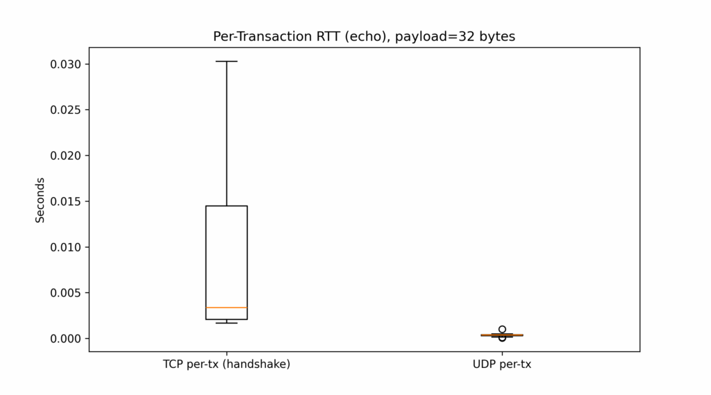
UDP consistently shows shorter durations due to its non-blocking, connectionless nature.
TCP introduces overhead from connection setup and acknowledgment processes.
In the async variant, latency is minimal with stable performance.
Limitations of the benchmark:
Tests run on localhost, eliminating real network congestion and packet loss
Real-world performance would differ significantly from these controlled conditions
For comprehensive UDP analysis, use tools like tc or netem on Linux to simulate jitter and packet loss
Secure Data Transmission in Healthcare IT
Medical data transmission (including electronic health records, lab results, imaging data, and wearable sensor streams) must meet strict requirements for confidentiality, integrity, availability, and traceability.
While TCP and UDP serve as foundational transport protocols, security and compliance in healthcare are implemented at higher layers through specialized protocols, encryption methods, and standardized frameworks designed specifically for medical contexts.
Key concepts
Transport-level security: Protocols like TLS (Transport Layer Security) establish encrypted communication channels over TCP connections, ensuring confidential and tamper-proof data transmission between endpoints. This security layer is commonly implemented in healthcare systems through protocols such as HTTPS for web-based applications and FTPS for secure file transfers, providing essential protection for sensitive patient information during network transit.
Application-level security: Healthcare standards such as HL7 v2, FHIR, and DICOM implement comprehensive security frameworks that utilize encrypted communication channels and enforce robust security measures including strict authentication protocols, granular role-based access control systems, and comprehensive audit logging mechanisms that track all data access and modifications for compliance and security purposes. These standards are designed to maintain data integrity while enabling secure information exchange between different healthcare systems and providers across organizational boundaries.
VPN/IPSec tunnels: These establish secure, encrypted communication pathways between healthcare facilities, including hospitals, outpatient clinics, laboratories, and remote patient monitoring devices. By creating protected virtual corridors across public networks, VPN/IPSec implementations ensure that sensitive medical data remains confidential and protected from unauthorized access during transmission, while maintaining compliance with healthcare privacy regulations and security standards.
Payload encryption: Medical data is often encrypted directly at the application level (using advanced symmetric encryption algorithms like AES-256 or asymmetric cryptographic methods such as RSA-2048) before transmission across any network. This additional security layer ensures that even if transport-level protections are compromised, the medical information itself remains encrypted and inaccessible to unauthorized parties, providing defense-in-depth for sensitive patient data regardless of the underlying transport protocol being used.
Protocols commonly used in medical systems
HL7 (Health Level 7): classic messaging for lab results, admissions, etc., often over TCP with MLLP framing, or over HTTPS (FHIR).
FHIR (Fast Healthcare Interoperability Resources): RESTful API standard using HTTP/HTTPS + JSON/XML + OAuth2 for secure access.
DICOM (Digital Imaging and Communications in Medicine): for imaging data (CT, MRI, ultrasound), built over TCP and optionally secured via TLS.
Standards, however, are a necessary but not sufficient condition. Two systems can both be FHIR-compliant and still fail to exchange anything clinically meaningful, because interoperability breaks down at the semantic and organisational level long before it breaks down at the protocol level.
Concrete technologies used in hospitals or medical software
Technology
Use
Security
VPN IPSec / OpenVPN
Inter-hospital connections or with remote devices
High
TLS 1.3 over HTTPS
FHIR or REST communications
High
SSH/SFTP
Secure transfer of HL7, CSV, XML files
High
DICOM over TLS
PACS/RIS communications
High (if enabled)
MQTT with TLS
Healthcare IoT, continuous monitoring devices
High
Mirth Connect
Integration engine for HL7/FHIR
Depends on configuration
Practical example: secure transmission of an ECG
ECG device captures patient data.
Data is formatted as XML or DICOM files.
The device creates a secure HTTPS/TLS connection with the central server.
The system verifies identity through OAuth2 authentication.
Encrypted data travels to either a FHIR API endpoint or an HL7 integration engine.
The server records the transaction and stores the data in an encrypted database.
Authorized physicians can view the data through a secure internal web portal (with authentication and comprehensive access logging).
Python for Medical Data Transfer
Let’s simulate the transmission of data with healthcare-grade security using HL7/FHIR protocols in Python. For this demonstration, we use the public HAPI FHIR Test Server, a free testing endpoint provided by the HAPI FHIR open-source project and maintained by Smile Digital Health. This server is designed exclusively for development and interoperability testing, with all uploaded resources being periodically purged. Never submit real patient data — use only synthetic or anonymized test data.
#--------------------# fhir transfer# di Michele Danilo Pierri# 08/08/2025#--------------------import requestsimport jsonimport uuidimport datetime# ------------------------# CONFIGURATION# ------------------------# Target FHIR server URL — for example, a test HAPI FHIR serverFHIR_SERVER_URL="https://hapi.fhir.org/baseR4/Patient"# Fake bearer token to simulate OAuth2 ACCESS_TOKEN="Bearer fake-token-for-demo-use-only"# ------------------------# FHIR RESOURCE GENERATION# ------------------------# Build a sample Patient resource according to the HL7 FHIR R4 standard# This object will be serialized as JSON and sent to the FHIR serverdefgenerate_fake_patient(): patient_id =str(uuid.uuid4()) # generate a random patient ID today = datetime.date.today().isoformat() patient_resource = {"resourceType": "Patient","id": patient_id,"active": True,"name": [ {"use": "official","family": "Doe","given": ["John"] } ],"gender": "male","birthDate": "1985-05-15","deceasedBoolean": False,"address": [ {"use": "home","line": ["1234 Main Street"],"city": "Springfield","state": "IL","postalCode": "62704","country": "USA" } ],"identifier": [ {"use": "usual","type": {"coding": [ {"system": "http://terminology.hl7.org/CodeSystem/v2-0203","code": "MR" } ] },"system": "http://hospital.smarthealth.org/mrn","value": f"MRN-{patient_id[:8]}" } ],"meta": {"lastUpdated": today } }return patient_resource# ------------------------# SENDING FUNCTION# ------------------------defsend_patient_to_fhir_server(patient_data):""" Sends the given FHIR Patient resource to the configured FHIR server using HTTPS POST. Includes authentication headers and content negotiation headers. """ headers = {"Authorization": ACCESS_TOKEN,"Content-Type": "application/fhir+json","Accept": "application/fhir+json" }try:print("Sending patient data to FHIR server...") response = requests.post(FHIR_SERVER_URL, headers=headers, data=json.dumps(patient_data))if response.status_code in [200, 201]:print("Patient resource successfully sent.")print(f"Server response location: {response.headers.get('Location', 'N/A')}")else:print(f"Failed to send patient resource. Status code: {response.status_code}")print(f"Response body: {response.text}")except requests.exceptions.RequestException as e:print(f"Network error: {e}")# ------------------------# MAIN# ------------------------if__name__=="__main__":print("Generating fake FHIR Patient resource...") patient = generate_fake_patient()print("Payload preview:")print(json.dumps(patient, indent=2)) send_patient_to_fhir_server(patient)
Technical notes
The HAPI server used accepts POST tests, but the data is public and visible to everyone.
In a real environment:
servers must use HTTPS with valid certificates;
authentication occurs through OAuth2 or JWT;
data must be encrypted at rest (not only in transit).
Legal and compliance framework
GDPR (EU): mandates encryption, access control, and data minimization.
HIPAA (US): requires secure transmission and auditability of health data.
ISO 27799 / ISO 27001: information security management in healthcare.
Practical Guidelines:
Use TCP when data integrity, delivery confirmation, and packet ordering are critical. This includes applications such as:
Clinical databases
Electronic health records (EHR)
DICOM imaging transfer between systems
Use UDP when real-time performance is more important than occasional packet loss, such as:
Telemedicine video streams
IoT patient monitoring devices
PACS viewers that preload images
Use asynchronous approaches (e.g. asyncio, aiohttp) when dealing with:
Multiple concurrent data streams (e.g. multi-patient monitoring)
Non-blocking UI-driven systems (e.g. healthcare dashboards)
Efficient use of network resources and low-latency systems
Secure all communication at the transport or application level:
Prefer HTTPS/TLS channels, even internally
Authenticate and authorize using OAuth2 or API keys
Log and audit every transaction involving personal data
Adopt medical standards such as FHIR and HL7 to ensure interoperability across systems, vendors, and national health infrastructures.
Conclusions
In this article, we examine the differences between TCP and UDP in terms of structure, behavior, and performance. Through practical benchmarking in Python, we demonstrated how these protocols behave under controlled conditions. We also extended our investigation to include asynchronous programming and its benefits in high-concurrency environments.
However, beyond theory and speed comparisons, we delved into the specific needs of healthcare IT, where the transmission of data is not just about speed or reliability, but about security, traceability, and compliance with international regulations.
Introduction: Why Build a Medical Database with Docker?
Creating a robust medical database system requires careful consideration of security, scalability, and maintainability. Furthermore, Docker containerization offers an ideal solution for healthcare applications by providing isolated environments that ensure consistent deployment across different systems.
In this comprehensive tutorial, we’ll explore how to create a medical database with Docker and perform operations on it using various tools. Additionally, we’ll use a practical example: a database designed to store patient demographic and anthropometric data (age, sex, height, weight, etc.).
While the structure we present is relatively simple, it can be scaled to accommodate more complex architectures. Moreover, this foundation provides the flexibility needed for future healthcare system expansions.
Building a medical database with Docker provides several advantages including isolation, portability, and ease of setup. First of all, Docker is an open-source tool for developing, distributing, and running software.
Its key feature is containerization—applications run in isolated environments that contain everything needed for the program to work. However, these containers share the host computer’s kernel while remaining isolated from its operating system. Think of them as lightweight virtual machines that are more efficient because they leverage the host’s kernel.
Thanks to isolation from the “host” environment, containers prevent conflicts from different dependencies and configurations. Consequently, they operate independently from the system while maintaining data persistence through mounted volumes.
SQLAlchemy: Simplifying Database Interactions
Next, SQLAlchemy is one of the most popular Python libraries for working with relational databases. It enables Python code to interact directly with various SQL databases through specific drivers, including MySQL, PostgreSQL, Oracle, and SQLite.
A key feature of SQLAlchemy is its Object-Relational Mapper (ORM), which maps database tables to Python classes. As a result, database interactions become straightforward and intuitive, reducing development time significantly.
Flask: Creating User-Friendly Web Interfaces
Flask is a Python framework for creating web applications. With Flask, we can build SQLAlchemy applications that access databases through an HTML interface. Therefore, users can interact with the medical database without requiring technical database knowledge.
With Docker running on your computer, you can download the MySQL database image from the terminal using this command:
dockerpullmysql:latest
This command downloads the latest MySQL image from the Docker Hub repository. Subsequently, once the image download is complete, we can create a container from it and configure it to meet our requirements.
Container Configuration and Setup
Navigate to the directory where you want to store your database (using standard commands like cd and mkdir). Then, run this script in the terminal:
–name: Sets the container’s name for easy identification
-v: Specifies the volume where data is stored, ensuring persistence
-e: Defines environment variables, including database credentials
-p: Specifies communication ports for external access
-d: Runs the container in detached mode
Managing Container Operations
These commands are only needed when initializing the container for the first time. After that, the specified parameters are saved and automatically applied whenever you run the container.
To verify the program has started successfully, use:
dockerps
Once you’ve created and configured the container, you won’t need to use docker run again. Instead, you’ll use different commands to stop and restart the program.
Furthermore, to manage your container operations use:
To stop the container:
dockerstopmy-mysql-container
To restart it, use:
dockerstartmy-mysql-container
To completely delete the container, use this command:
dockerrm-fmy-mysql-container
Note: An alternative method called docker compose lets you manage container configurations through a docker-compose.yml file. This approach is typically used for applications with multiple containerized programs, but we won’t cover it in this tutorial.
Step 2: Creating Database Tables with SQLAlchemy
Environment Setup and Library Installation
It is recommended to use an IDE (like Visual Studio Code) and create a virtual environment to complete this step; you also need to verify that the container is active or activate it with the command:
dockerstartmy-mysql-container
From Visual Studio Code’s terminal, install the required Python libraries:
Create an engine to connect to the database. The engine manages the connection pool and database access. Setting echo=True enables SQL statement logging for debugging.
engine = create_engine(DATABASE_URL, echo=True)
SQLAlchemy uses a foundational “base” class that helps create database tables in Python. This base class acts as a template – when you create new table classes, they inherit from this base class, making it simple to define and work with database tables in your Python code.
To define it, we use the command:
Base = declarative_base()
Designing Patient Records Table
Now let’s create the first table, the patient’s PatientRecords using SQLAlchemy’s Base class as a template:
classPatientRecords(Base): __tablename__ ='patient_records'# Table name in the database# Columns Id_patient = Column(Integer, primary_key=True, autoincrement=True) # Primary key first_name = Column(String(50), nullable=False) # Patient's first name last_name = Column(String(50), nullable=False) # Patient's last name date_of_birth = Column(Date, nullable=False) # Patient's date of birth# Relationship with the "AnthropometricData" table anthropometric_data = relationship("AnthropometricData", back_populates="patient")def__repr__(self):returnf"<PatientRecords(Id_patient={self.Id_patient}, first_name={self.first_name}, last_name={self.last_name})>"
In this script, we define both the table name (patients_record) and its fields, while also establishing a relationship with the Anthropometric_data table (relationship = AnthropometricData). This relationship is bidirectional (back_populates = “patient”). When we create the Anthropometric_data table, we’ll set up a corresponding PatientRecord relationship with a bidirectional link (back_populates = AnthropometricData) to the Patient_record table.
This creates a “logical” link between the two tables, complementing the structural connection already established through Foreign Keys at the database level.
The repr(self) method defines how an object should be represented when it is printed or displayed, converting it into a more readable string format.
Creating Anthropometric Data Table
Let’s create the second table (antropometric_data) using the same approach we used for the PatientRecords table.
classAnthropometricData(Base): __tablename__ ='anthropometric_data'# Table name in the database# Columns Id_data = Column(Integer, primary_key=True, autoincrement=True) # Primary key Id_patient = Column(Integer, ForeignKey('patient_records.Id_patient'), nullable=False) # Foreign key to "patient_records" height = Column(Float, nullable=False) # Height in cm weight = Column(Float, nullable=False) # Weight in kgBMI= Column(Float, nullable=False) # Body Mass Index (calculated as weight / (height/100)^2)# Relationship with the "PatientRecords" table patient = relationship("PatientRecords", back_populates="anthropometric_data")def__repr__(self):returnf"<AnthropometricData(Id_data={self.Id_data}, Id_patient={self.Id_patient}, BMI={self.BMI})>"
It’s important to note that, at this point, the tables exist only as logical definitions and haven’t been created in the actual database. The following command will transform them into real tables in our archive by converting our logical structure into SQL commands. SQLAlchemy handles this conversion automatically, saving us significant effort.
Base.metadata.create_all(engine)
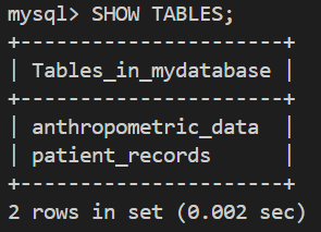
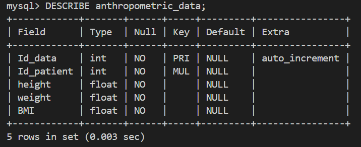
To verify that the tables were successfully created, you can interact directly with the MySQL database through the terminal with these commands:
docker exec-it my-mysql-container mysql -u myuser -pUSE mydatabase;SHOWTABLES;DESCRIBE patient_records;DESCRIBE anthropometric_data;
These commands will display the following:
Step 3: Data Operations and Management
Session Management and Database Operations
After setting up the database and tables, we can proceed to populate them with content.
If you create a new program to perform database operations, you’ll need to include the table class definitions (PatientRecords and AnthropometricData) again. While you can copy these definitions manually, there are more efficient ways to avoid this duplication, though we’ll keep things simple and won’t cover those techniques here.
In order to perform database operations (such as queries and data insertion) with SQLAlchemy, we first need to use sessionmaker.
Rolling back changes if errors occur (session.rollback())
Closing the session (session.close())
Adding Patient Records
Now that we have created a session, we can add a new patient to the patient_records table:
new_patient = PatientRecords(first_name="Mario",last_name="Rossi",date_of_birth="1990-05-15"# Date format: YYYY-MM-DD)session.add(new_patient)session.commit()
Note that we insert the new patient using the Python table class (PatientRecords) rather than the actual table name (patient_records). SQLAlchemy provides this layer of abstraction, letting us focus on logical operations instead of directly referencing table names. Behind the scenes, SQLAlchemy converts our code into SQL instructions to interact with the database.
Managing Anthropometric Data
Next, let’s add data to the anthropometric_data table:
anthropometric_data = AnthropometricData(Id_patient=new_patient.Id_patient,height=175.0, # Height in cmweight=70.0, # Weight in kgBMI=70.0/ ((175.0/100) **2) # Calculate BMI)session.add(anthropometric_data)session.commit()
Querying and Verification
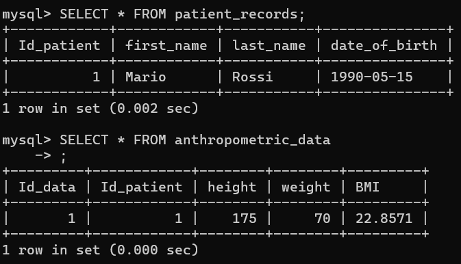
Let’s query the tables to verify that our data was successfully inserted:
patients = session.query(PatientRecords).all()print("\\nPatients in the database:")for patient in patients:print(patient)anthropometric_records = session.query(AnthropometricData).all()print("\\nAnthropometric Data in the database:")for record in anthropometric_records:print(record)
Finally, let’s close the session:
session.close()
Alternatively, you can query the database directly through Docker using SQL commands in the terminal:
Our medical database project will use three HTML templates as the foundation for interacting with the container:
index.html – the main page
add_patient.html – for adding new patients
edit_patient.html – for modifying patient records
Directory Structure and Organization
The directory organization will be:
flask_app/│├── app.py # Main Flask app file├── models.py # ORM class definitions (PatientRecords, AnthropometricData)├── templates/ # HTML templates folder│ ├── index.html # Main page│ ├── add_patient.html # Form to add a patient└ └── edit_patient.html# Form to modify a patient
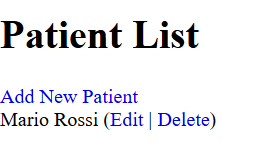
We’ll create three HTML templates. The first (index.html) serves as the entry page, displaying the database content and allowing users to select various operations.
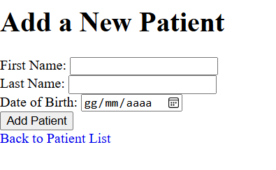
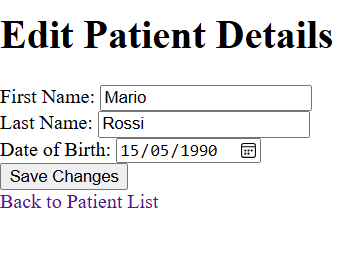
The second page (add_patient.html) provides a form for adding patients to the patient_records dataset, while the third page (edit_patient.html) enables modification of existing patient data.
At this stage, we’ve prioritized system functionality over aesthetics, though the visual aspects can be easily improved later.
The script for index.html:
<!DOCTYPEhtml><html><head> <title>Patient List</title></head><body> <h1>Patient List</h1><!-- Link to add a new patient --> <ahref="{{ url_for('add_patient') }}">Add New Patient</a> <ul><!-- Loop through all patients and display their details --> {% for patient in patients %} <li> {{ patient.first_name }} {{ patient.last_name }}<!-- Links to edit or delete the patient --> (<ahref="{{ url_for('edit_patient', patient_id=patient.Id_patient) }}">Edit</a> | <ahref="{{ url_for('delete_patient', patient_id=patient.Id_patient) }}">Delete</a>) </li> {% endfor %} </ul>
The script for add_patient.html:
<!DOCTYPEhtml><html><head> <title>Add Patient</title></head><body> <h1>Add a New Patient</h1><!-- Form to submit new patient details --> <formmethod="POST"> First Name: <inputtype="text"name="first_name"><br> Last Name: <inputtype="text"name="last_name"><br> Date of Birth: <inputtype="date"name="date_of_birth"><br> <buttontype="submit">Add Patient</button> </form><!-- Link to return to the patient list --> <ahref="{{ url_for('index') }}">Back to Patient List</a></body></html>
The script for edit_patient.html:
<!DOCTYPEhtml><html><head> <title>Edit Patient</title></head><body> <h1>Edit Patient Details</h1><!-- Form to update patient details --> <formmethod="POST"> First Name: <inputtype="text"name="first_name"value="{{ patient.first_name }}"><br> Last Name: <inputtype="text"name="last_name"value="{{ patient.last_name }}"><br> Date of Birth: <inputtype="date"name="date_of_birth"value="{{ patient.date_of_birth }}"><br> <buttontype="submit">Save Changes</button> </form><!-- Link to return to the patient list --> <ahref="{{ url_for('index') }}">Back to Patient List</a></body></html>
Flask Application Development
The app.py program follows below. The program uses Flask decorators (marked by “@app.route()”) to connect web pages with Python code, managing database requests and responses.
from flask import Flask, render_template, request, redirect, url_forfrom sqlalchemy import create_enginefrom sqlalchemy.orm import sessionmakerfrom models import PatientRecords, AnthropometricData# Database configurationDATABASE_URL="mysql+pymysql://myuser:mypassword@localhost:3306/mydatabase"engine = create_engine(DATABASE_URL) # Create a connection to the databaseSession = sessionmaker(bind=engine) # Create a session factorysession = Session() # Initialize a session to interact with the database# Initialize Flask appapp = Flask(__name__)# Home Page: Display all patients@app.route("/")defindex(): patients = session.query(PatientRecords).all() # Query all patients from the databasereturn render_template("index.html", patients=patients) # Render the template with patient data# Add Patient Page: Handle form submission to add a new patient@app.route("/add", methods=["GET", "POST"])defadd_patient():if request.method =="POST":# Retrieve form data first_name = request.form["first_name"] last_name = request.form["last_name"] date_of_birth = request.form["date_of_birth"]# Create a new patient object new_patient = PatientRecords(first_name=first_name,last_name=last_name,date_of_birth=date_of_birth ) session.add(new_patient) # Add the new patient to the session session.commit() # Commit the transaction to save the datareturn redirect(url_for("index")) # Redirect to the home pagereturn render_template("add_patient.html") # Render the form for GET requests# Edit Patient Page: Handle form submission to update an existing patient@app.route("/edit/<int:patient_id>", methods=["GET", "POST"])defedit_patient(patient_id): patient = session.query(PatientRecords).get(patient_id) # Retrieve the patient by IDif request.method =="POST":# Update patient details with form data patient.first_name = request.form["first_name"] patient.last_name = request.form["last_name"] patient.date_of_birth = request.form["date_of_birth"] session.commit() # Commit the changes to the databasereturn redirect(url_for("index")) # Redirect to the home pagereturn render_template("edit_patient.html", patient=patient) # Render the edit form# Delete Patient Page: Delete a patient by ID@app.route("/delete/<int:patient_id>")defdelete_patient(patient_id): patient = session.query(PatientRecords).get(patient_id) # Retrieve the patient by ID session.delete(patient) # Delete the patient from the session session.commit() # Commit the transaction to apply the deletionreturn redirect(url_for("index")) # Redirect to the home page# Run the Flask appif__name__=="__main__": app.run(debug=True) # Start the app in debug mode for development
The initial page displays the database records and all available actions that can be performed on them:
The additional pages enable users to add or modify patient records:
Step 5: Critical Security Considerations
Understanding Healthcare Data Protection
We are dealing with a medical database and therefore sensitive data whose protection is regulated by legislation. Moreover, GDPR (General Data Protection Regulation) in Europe and HIPAA (Health Insurance Portability and Accountability Act) in the United States impose strict requirements.
Identifying Security Vulnerabilities
Even with a superficial analysis, we can identify numerous critical issues in the structure we have built:
Exposed passwords: Access credentials to the dataset are embedded in the code and therefore easily stolen.
Unauthenticated access: The Flask application lacks authentication mechanisms for HTML pages.
Unencrypted data: Data transmission between the Flask server and HTML pages is not encrypted.
SQL injection vulnerability: Input data is not validated, exposing the system to attacks through harmful SQL commands.
Cross-Site scripting vulnerability: Malicious users could exploit the web interface to inject harmful scripts.
Database exposure: The database is accessible on port 3306: if this port is public, it could be targeted for direct attacks.
Implementing Security Measures
Solutions to these issues include:
Environment variable management for credentials
Authentication middleware implementation
HTTPS encryption for data transmission
Input validation and parameterized queries
Content Security Policy headers
Network segmentation and firewall rules
Step 6: Summary and Next Steps
Key Concepts Review
Let’s summarize the key concepts covered in this tutorial:
First, we used Docker to create a MySQL container, providing an isolated and configurable medical database environment. Subsequently, we implemented SQLAlchemy as an ORM to map database tables to Python classes. Finally, we built a Flask web application that enables browser-based database interactions.
Future Development Possibilities
While this structure is straightforward, it serves as a robust foundation. Furthermore, it can be expanded into more complex architectures including:
Multi-container orchestration with Docker Compose
Advanced authentication and authorization systems
Real-time data synchronization capabilities
Comprehensive audit logging mechanisms
Integration with Electronic Health Record (EHR) systems
Scaling Considerations
As your medical database grows, consider implementing:
Database indexing strategies for improved performance
Caching mechanisms for frequently accessed data
Load balancing for high-availability deployments
Backup and disaster recovery procedures
Compliance monitoring and reporting tools
Conclusion: Building Secure Healthcare Systems
This tutorial has provided a comprehensive foundation for building medical databases with Docker. However, remember that production healthcare systems require additional security measures and compliance considerations.
Therefore, always consult with security professionals and legal experts when handling sensitive medical data. Additionally, stay updated with the latest security best practices and regulatory requirements in your jurisdiction.
In a previous blog post, we explored how to read the content of a DICOM file, including its numerous tags. These tags provide insights into the study type, characteristics, and all relevant patient and study information.
Now, we’ll focus on the most crucial tag—the one containing the images. A typical study can include anywhere from a few to several hundred DICOM files, usually identifiable by their .dcm extension.
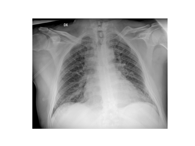
For our practice, we’ll open a single .dcm file containing a frontal projection chest X-ray.
Environment Setup
Before we begin, it’s essential to install some key libraries. Due to dependency issues, it’s best to create a dedicated environment for running Python with these libraries. In our environment, we’ve installed numpy, pandas, and matplotlib—common libraries for data management and visualization—as well as the pydicom library discussed in our previous post.
For this specific task, we’ve also installed these additional libraries:
scipy: An open-source library for scientific computing in Python, based on numpy. It’s particularly useful for applying image transformation filters.
opencv (cv2): The Open Source Computer Vision Library, which uses machine learning for computer vision tasks. It provides various tools for image processing. In Python, you can access it through the cv2 module.
pylibjpeg, pylibjpeg-libjpeg, and gdcm: These libraries are necessary for working with and processing DICOM files.
Our radiographic image is located at IMAGES\01\00001.dcm on a diagnostic CD. It contains a frontal projection chest X-ray. The same directory also includes file 00002.dcm, which contains the lateral projection—we won’t be using this for now.
Loading the image
First, let’s import the necessary libraries:
import pydicomimport matplotlib.pyplot as pltimport numpy as np
Now, we’ll locate our .dcm file and load the dataset into the dicom_data variable.
The image data in dicom_data is stored in the pixel_array attribute, which we’ll assign to the image variable. This creates a numpy array of rows and columns containing the pixel data that forms the image.
# Specify the path to the DICOM filedicom_path ="C:\\Dicom\\RX\\IMAGES\\01\\00001"# Read the DICOM filedicom_data = pydicom.dcmread(dicom_path)# Extract the image from the DICOM datasetimage = dicom_data.pixel_array:
Let’s extract some key information about our image: its data type, dimensions in pixels, and the range of possible pixel values:
# Information about the arrayprint("Pixel data type:", image.dtype)print("Image dimensions:", image.shape)print("Maximum pixel value:", np.max(image))print("Minimum pixel value:", np.min(image))
Pixel data type: uint16 Image
dimensions: (2400, 2880)
Maximum pixel value: 4095
Minimum pixel value: 0
Our image has dimensions of 2400 x 2880 pixels, with each pixel capable of holding a value from 0 to 4095.
The pixel data type indicates a bit depth of 16 unsigned bits (u) per pixel, allowing for 2^16 = 65,536 grayscale values (opacity and brightness) ranging from 0 to 65,535. In contrast, an 8-bit image has a lower depth, with each value on the scale ranging from 0 to 255 (2^8 = 256 values).
However, it’s worth noting that while the data type allows for up to 65,535 values, the actual image in this case only uses values from 0 to 4095. This suggests that the image is effectively using 12 bits of information (2^12 = 4096 possible values), even though it’s stored in a 16-bit format.
Medical images are typically stored in 12- or 16-bit formats. The lowest values (0) correspond to darker areas in the image.
We can visualize the image using matplotlib:
# Display the imageplt.imshow(image, cmap="gray")plt.axis("off") # Hide axes for a clean visualizationplt.show()
The resulting image will be displayed as follows:
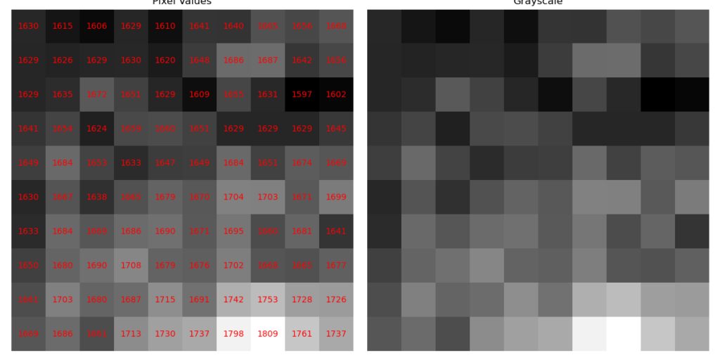
Out of curiosity, let’s extract the values from a small 10×10 pixel area of the image, read the stored values, and reconstruct them based on the grayscale.
# Define the starting position for the square (you can modify it based on your needs)start_x, start_y =100, 100# For example, the top-left pixel of the square# Extract a 10x10 pixel square from the resized frontal imagesquare = image[start_y:start_y+10, start_x:start_x+10]# Display the numerical values of the pixelsfig, axes = plt.subplots(1, 2, figsize=(12, 6))# First grid: numerical pixel valuesaxes[0].imshow(square, cmap="gray")for i inrange(10):for j inrange(10):# Insert the pixel value at the center of the cell axes[0].text(j, i, int(square[i, j]), ha="center", va="center", color="red", fontsize=10)axes[0].set_title("Pixel Values")axes[0].axis("off") # Remove axes for a clean visualization# Second grid: grayscaleaxes[1].imshow(square, cmap="gray")axes[1].set_title("Grayscale")axes[1].axis("off")# Optimize the layoutplt.tight_layout()plt.show()
Various operations can be performed on the pixel matrix that composes the image. Let’s explore a few of them.
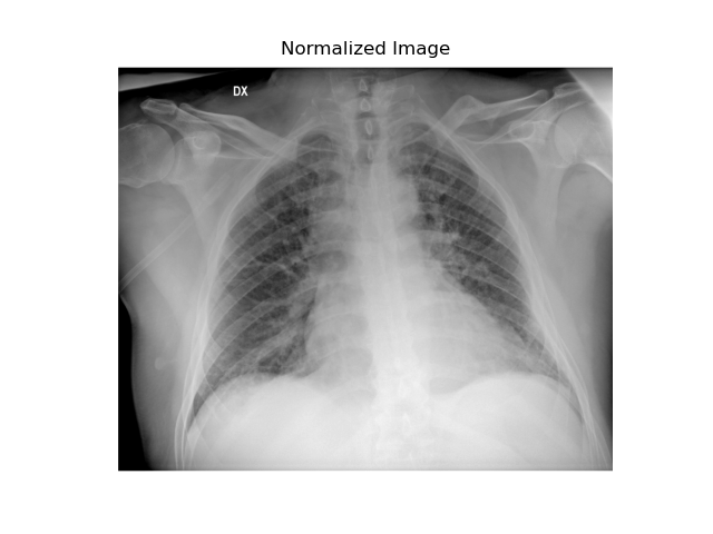
Normalization
When the grayscale range is extensive (in our case, from 0 to 65,535), it’s often beneficial to normalize it to a scale of 0 to 255. This process can enhance the visibility of details perchè con valori di intensità molto distanti potrebbero essere non distinguibili.
When the grayscale range is extensive (in our case, from 0 to 65,535), it’s often beneficial to normalize it to a scale of 0 to 255. This process can enhance the visibility of details, as intensity values that are very far apart might otherwise be indistinguishable to the human eye.
# Normalization between 0 and 255image_normalized = (image - np.min(image)) / (np.max(image) - np.min(image)) *255image_normalized = image_normalized.astype(np.uint8)# Display the normalized imageplt.imshow(image_normalized, cmap="gray")plt.title("Normalized Image")plt.axis("off")plt.show()
Equalization
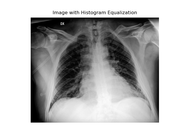
This technique adjusts pixel values to better distribute intensities across the image. It’s particularly useful for radiographic images as it enhances the visibility of structures that are otherwise difficult to perceive.
To perform equalization, we’ll use the cv2 library:
import cv2# Histogram equalization with OpenCVimage_equalized = cv2.equalizeHist(image_normalized)plt.imshow(image_equalized, cmap="gray")plt.title("Image with Histogram Equalization")plt.axis("off")plt.show()
Smoothing or Gaussian Filter
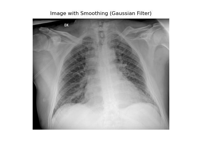
The Gaussian filter averages nearby pixels to reduce sudden value variations and noise. As a result, images appear less detailed but more uniform.
You can import the Gaussian filter from scipy.
from scipy.ndimage import gaussian_filter# Apply a Gaussian filter to reduce noiseimage_smoothed = gaussian_filter(image_normalized, sigma=1)# Display the image with smoothingplt.imshow(image_smoothed, cmap="gray")plt.title("Image with Smoothing (Gaussian Filter)")plt.axis("off")plt.show()
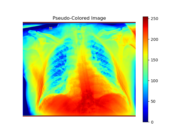
Pseudocoloring
Pseudocoloring applies filters to colorize areas in grayscale images, enhancing visual analysis. For instance, the “jet” filter assigns blue to low intensities and red to high intensities, making different regions more distinguishable.
# Apply a "jet" color map for pseudo-coloringplt.imshow(image_normalized, cmap="jet")plt.title("Pseudo-Colored Image")plt.axis("off")plt.colorbar() # Add a color bar for referenceplt.show()
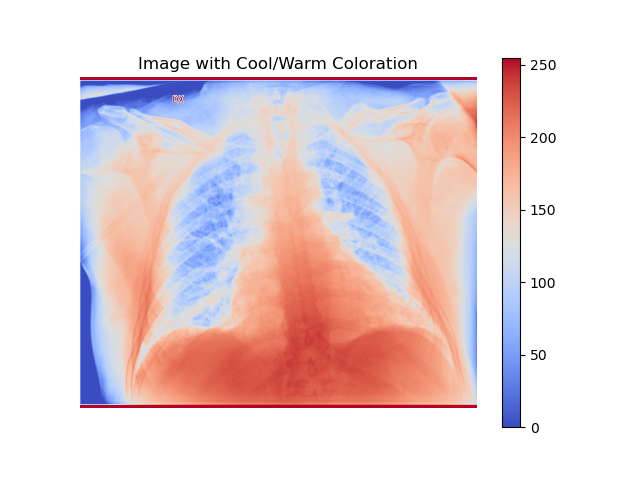
Another color scale option is the cool/warm scale:
plt.imshow(image_normalized, cmap="coolwarm")plt.title("Image with Cool/Warm Coloration")plt.axis("off")plt.colorbar()plt.show()
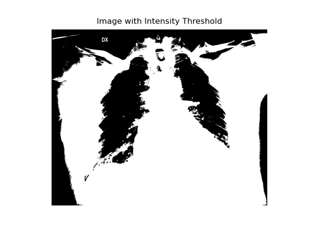
Thresholding
The image is converted to binary, with pixels below a certain threshold becoming black and those above turning white. This process highlights high-density elements like bones in an X-ray.
threshold_value =128# Example threshold, to be adapted to the imageimage_thresholded = (image_normalized > threshold_value) *255plt.imshow(image_thresholded, cmap="gray")plt.title("Image with Intensity Threshold")plt.axis("off")plt.show()
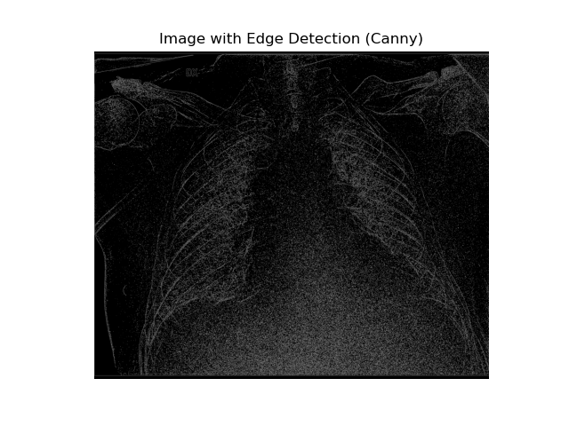
Edge Detection (Canny)
The Canny edge detection algorithm identifies edges in an image based on intensity gradients. It uses two threshold values to determine which edges to keep.
# Apply edge detection using OpenCV's Canny methodedges = cv2.Canny(image_normalized, threshold1=30, threshold2=34)# Display the detected edgesplt.imshow(edges, cmap="gray")plt.title("Image with Edge Detection (Canny)")plt.axis("off")plt.show()
Thresholding and edge detection share a limitation: they separate structures on the basis of pixel intensity alone, with no notion of what the structure actually is. A bone edge and a catheter edge look the same to Canny. Identifying which pixels belong to a given anatomical structure requires semantic segmentation, and the reference architecture for medical images is UNet, designed precisely to work with the small annotated datasets that clinical research typically produces.
With the pixel matrix that composes an image at our disposal, we have a wide array of manipulation techniques to enhance its visualization. These techniques allow us to extract more information, highlight specific features, or improve the overall clarity of the image.
In many medical imaging scenarios, we often encounter multiple images of the same patient and anatomical region. This presents exciting opportunities beyond single-image manipulation. We can use these multiple images to reconstruct three-dimensional volumes, providing a more comprehensive view of the anatomy. Additionally, we can create dynamic sequences or moving images, which can be particularly useful for studying physiological processes or changes over time.
These advanced processing techniques, such as volume reconstruction and dynamic imaging, open up new possibilities for diagnosis, treatment planning, and medical research. They allow healthcare professionals to gain deeper insights into patient anatomy and physiology, potentially leading to more accurate diagnoses and improved patient care
DICOM stands for Digital and Communications in Medicine and is used for managing medical data. One of the most common uses of this format is the storage, transfer, and display of diagnostic images like X-rays, CT scans, and MRIs.
While there are variations depending on the type of image and the manufacturer of the equipment that generated it, a DICOM file contains some common elements:
HEADER: The initial part of the file contains metadata describing its content (patient identification, image acquisition modality, parameters for acquiring the images, equipment manufacturer, etc.).
ATTRIBUTE GROUPS: The metadata in the header is organized into attribute groups containing a series of DICOM tags that provide specific information. For example, tag 0010,0010 specifies the patient’s name.
TRANSFER SYNTAX: Specifies how the data is encoded and stored.
IMAGE: Contains the pixels or voxels that make up the image, which may be compressed or uncompressed.
TRAILER: Indicates the end of the DICOM file and may be absent.
The main attributes of a DICOM file include:
PatientName: Patient’s name.
PatientAge: Patient’s age.
StudyDate: Date of the study.
StudyDescription: Study description.
Modality: Imaging modality used (e.g., CT, MR, X-ray, etc.).
Manufacturer: Imaging equipment manufacturer.
Rows: Number of rows in the image.
Columns: Number of columns in the image.
PixelData: Image pixel data.
ImageOrientationPatient: Image orientation relative to the patient.
ImagePositionPatient: Spatial position of the image relative to the patient.
SliceThickness: Slice thickness in an imaging volume.
PixelSpacing: Pixel spacing in the image.
When examining a DICOM file related to angiographic images, the modality will be XA. The study type attribute will specify whether it is coronary, cerebral, or another type of angiography. The sequence type attribute indicates the direction of the subsequent images (anteroposterior, lateral, oblique). The number of images in the sequence is usually indicated by the “NumberOfFrames” tag.
A very useful library for working with DICOM files in Python is pydicom. It is the one we will use for all work on DICOM files.
Before accessing it, you need to install it by running the following command in the terminal:
pipinstallpydicom
The following program reads the attributes of the DICOM (.dcm) file specified in the “dicom_file_path” variable.
import pydicomdefprint_dicom_attributes(dicom_file):# Load the DICOM file ds = pydicom.dcmread(dicom_file)# Iterate over all data elements in the DICOM datasetfor element in ds:# Extract the tag, name, and value of the DICOM attribute tag = element.tag name = element.name# Print the attribute informationprint(f"Tag: {tag}, Name: {name}")if__name__=="__main__":# Specify the path to the DICOM file dicom_file_path ="path/to/your/dicom/file.dcm"# Call the function to print DICOM attributes print_dicom_attributes(dicom_file_path)
The list of attributes obtained is often very long and not very useful.
We can limit the number of attributes to those we are interested in and read their contents. In the following program, we created a dictionary containing some specific attributes and read them:
import pydicomdefprint_important_dicom_attributes(dicom_file):# Load the DICOM file ds = pydicom.dcmread(dicom_file)# Define a list of important tags to print important_tags = {"PatientName": "Patient's Name","PatientID": "Patient's ID","PatientBirthDate": "Patient's Birth Date","PatientSex": "Patient's Sex","StudyID": "Study ID","StudyDate": "Study Date","StudyTime": "Study Time","SeriesNumber": "Series Number","Modality": "Modality","Rows": "Number of Rows in Image","Columns": "Number of Columns in Image","NumberOfFrame": "Number of Frames in Sequence }# Iterate over the important tags and print their valuesfor tag, description in important_tags.items():if tag in ds: value = ds.data_element(tag).valueprint(f"{description} ({tag}): {value}")else:print(f"{description} ({tag}): Not Available")if__name__=="__main__":# Specify the path to the DICOM file dicom_file_path ="path/to/your/dicom/file.dcm"# Call the function to print important DICOM attributes print_important_dicom_attributes(dicom_file_path)
The output is as follows:
Patient’s Name (PatientName): XXXXXX^XXXXXX
Patient’s ID (PatientID): 000000000000000000
Patient’s Birth Date (PatientBirthDate): 19000402
Patient’s Sex (PatientSex): M
Study ID (StudyID): 2020000
Study Date (StudyDate): 20200000
Study Time (StudyTime): 084611.000
Series Number (SeriesNumber): 1
Modality (Modality): XA
Number of Rows in Image (Rows): 512
Number of Columns in Image (Columns): 512
Number of Frames in Sequence (NumberOfFrames): 86
In an upcoming article, we will delve into the part of the file containing the image pixels to view and manage them.
Python has become an increasingly vital tool for analyzing healthcare data. It is a widely used programming language. According to the PYPL (Popularity of Programming Language) index, it ranks as the world’s most popular programming language, commanding a 30.7% market share. By comparison, Java holds 14.89% and JavaScript 7.78% of the market.
Python’s success stems from its power, versatility, and user-friendly design. With its clear, readable syntax and gentler learning curve compared to other languages, Python is accessible to many users.
Its multi-paradigm nature — supporting imperative, functional, and object-oriented programming — lets developers choose the most suitable approach for each task.
Furthermore, an active developer community has created extensive libraries and frameworks that enhance Python’s capabilities and ease of use.
With powerful libraries like TensorFlow, Keras, and Scikit-learn, Python has become the preferred language for machine learning and artificial intelligence development.
When properly implemented following best practices, these Python libraries can analyze healthcare data to enhance patient diagnosis and treatment outcomes.
In this article, we will briefly explore how to use Python to analyze healthcare data, covering the entire process from data import to results visualization.
Essential Python Libraries for Healthcare Data Management
Numpy and Pandas
These areare two essential Python libraries for data analysis, each with complementary functionalities particularly useful in healthcare.
NumPy provides the mathematical foundation for scientific computing in Python through high-performance multidimensional arrays and numerous mathematical functions that enable efficient complex calculations. This library allows for biomedical signal processing, diagnostic image analysis, and supports advanced statistical algorithms necessary for interpreting clinical data.
Pandas, on the other hand, focuses on structured data manipulation and analysis through its main data structures, DataFrame and Series, which greatly facilitate working with tabular information. In healthcare, Pandas excels in managing electronic health records, epidemiological data, and time series of clinical parameters, offering robust functionality for data cleaning, handling missing values, and information aggregation.
These two libraries are typically used in combination: NumPy provides the computational power necessary for underlying mathematical operations, while Pandas offers an intuitive interface to manipulate and explore healthcare datasets, enabling researchers and industry professionals to extract meaningful information, identify trends in patient data, and develop predictive models to improve diagnosis and treatments.
Pyhealth
Pyhealth is a specialized library for developing machine learning applications in healthcare. It supports major medical databases like MIMIC-III, MIMIC-IV, and eICU, providing base outputs for MIMIC-III. The library includes templates for key predictions such as readmission risk, length of stay, and treatment recommendations. It enables users to build predictive models and evaluate their performance. The library also supports over 20 medical coding systems, including ICD-9 and ICD-10, for diagnoses, treatments, and medications.
Lifelines
Lifelines is a tool for survival analysis using various techniques, including Kaplan-Meier, Nelson-Aalen, and regression. It covers most parametric and non-parametric methods and supports the creation of related graphs. Lifelines features an intuitive design and a scikit-learn-like API, making it easily accessible to data scientists and researchers who are already familiar with Python’s ecosystem.
Biopython
BioPython is a powerful tool for analyzing molecular and computational biology. The library streamlines common bioinformatics tasks, enabling researchers to concentrate on interpreting results instead of managing data.
Nilearn
Nilearn is a Python library for neuroimaging analysis and visualization built on scikit-learn. It is an essential tool for neuroscientists and researchers working with neuroimaging data, especially functional magnetic resonance imaging (fMRI).
By connecting traditional neuroimaging analysis with machine learning, Nilearn makes advanced statistical techniques more approachable for neuroscientists. Its comprehensive documentation, complete with tutorials and examples, ensures accessibility even for newcomers to the field.
The library integrates with Python’s scientific ecosystem—including NumPy, SciPy, Matplotlib, and scikit-learn—enabling efficient workflows in neuroscientific research.
Pymedtermino
It is a useful library for managing medical terminology. It supports various standards like ICD-10 and is beneficial for coding and analyzing healthcare data.
Pymc
Pymc is a package for running models based on Bayesian statistics, ideal for building healthcare models like predicting outcomes.
Libraries based on FHIR
FHIR (Fast Healthcare Interoperability Resources) is a standard developed by HL7 (Health Level Seven) for exchanging healthcare information between various systems and devices. Several Python packages are available for working with FHIR: Fhir.resources – Google-fhir-py – Fhirpack
Libraries for Medical Image Visualization
A crucial aspect of healthcare applications is managing and visualizing medical images. Python libraries are numerous and vital for creating these visual applications:
Matplotlib
Though not specifically designed for image visualization, Matplotlib excels in creating and displaying 2D and 3D graphs and images.
ITK
ITK is a tool that enables multidimensional image analysis and segmentation, especially for CT or MRI images. It also allows the alignment of images from various sources. SimpleITK, built on ITK, offers numerous image manipulation tools. These tools are powerful and widely used.
Medpy
Medpy is a collection of scripts that lets you manipulate, read, and write medical images in Python. Based on SimpleITK, Medpy supports numerous formats, from DICOM to those of the Neuroimaging Informatics Technology Initiative, Nrrd, MINC, GIPL, microscopic images, PNG, JPG, JPEG, TIFF, BMP, and more. It also enables feature extraction for use in machine learning programs like Scikit-Learn.
Scikit-image
It’s a collection of algorithms for image processing.
Pydicom
Pydicom is a Python library for working with DICOM files—reading, manipulating, and saving them. As a native Python application, it is easy for users to utilize.
To use these libraries in Python, you need to first install them on your system and then import them into your code. We recommend installing in a virtual environment, as shown in other articles on this blog.
Typically, installation is done by typing in the terminal, in pip environment:
pipinstallnamelibrary
In Conda environment:
condainstall-cconda-forgenamelibrary
Generally, libraries installed with pip and those installed in a Conda environment are separate and not automatically accessible to each other. This difference arises because pip and Conda manage environments and dependencies differently. If you use both environments, it is advisable to perform both installations.
Some libraries need specific commands for installation. You can find detailed instructions on their respective linked Pyp pages.
After the installation is complete, you can import the library into your projects using the import statement:
import namelibrary ## or, if use with aliasimport namelibrary as alias