
Introduction
K-nearest Neighbors (KNN) is one of the most powerful and widely used algorithms in Machine Learning. While it can handle classification and regression tasks, it’s primarily used for classification. This focus on classification arises from the availability of more efficient algorithms for regression problems.
Definition
K-Nearest Neighbors is a non-parametric model that works by finding similarities. It follows a simple principle: in an ideal feature space, similar objects naturally group together. We can identify an object’s category by examining how close it is to other objects.
This is why measuring distances, as covered in the previous chapter, is essential.
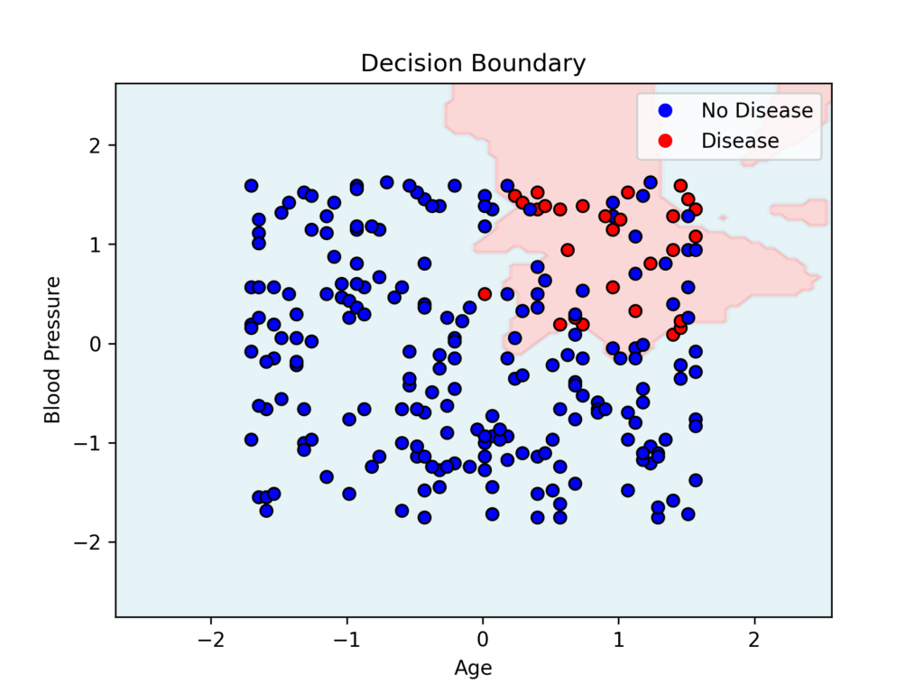
The decision boundary marks the line of separation between classes in the feature space.
Medical Applications
KNN has several important applications in medicine:
Patient diagnosis through comparison of characteristics to identify conditions like diabetes
Classification of skin lesions through image comparison with labeled samples
Analysis of CT scans by comparing them with labeled images to detect cancer
The following medical publications demonstrate the use of this algorithm:
Saini I, Singh D, Khosla A. K-nearest neighbour-based algorithm for P- and T-waves detection and delineation. J Med Eng Technol. 2014 Apr;38(3):115-24. doi: 10.3109/03091902.2014.882424. Epub 2014 Feb 10. PMID: 24506210.
Siddalingappa R, Kanagaraj S. K-nearest-neighbor algorithm to predict the survival time and classification of various stages of oral cancer: a machine learning approach. F1000Res. 2023 Nov 16;11:70. doi: 10.12688/f1000research.75469.2. PMID: 38046542; PMCID: PMC10690040.
Uddin S, Haque I, Lu H, Moni MA, Gide E. Comparative performance analysis of K-nearest neighbour (KNN) algorithm and its different variants for disease prediction. Sci Rep. 2022 Apr 15;12(1):6256. doi: 10.1038/s41598-022-10358-x. PMID: 35428863; PMCID: PMC9012855.
Indications for Using KNN
KNN doesn’t assume any specific data distribution pattern, making it suitable for non-linear relationships between variables. For example, it works well for tumor classification using radiographic or histological images.
KNN performs best with small datasets, as it becomes less efficient with larger ones.
The algorithm requires numerical and scaled data. If your data uses different scales, you must normalize or standardize it first.
KNN offers intuitive and easily interpretable results, making it accessible even to non-experts in data analysis.
The algorithm works best when classes are clearly separated. For overlapping classes, other classification methods are more appropriate.
Limitations of Using KNN
With large datasets (n > 100,000), KNN becomes inefficient since it must calculate distances between all observation pairs.
If there are many features, Euclidean distance loses meaning (see curse of dimensionality)
Outliers and anomalous data can significantly affect predictions
The algorithm is slow during prediction because it must compare all data points, making it unsuitable when speed is crucial.
KNN Application in Python
Like all Machine Learning algorithms, proper dataset preparation is essential:
Features must be numerical, and data must be clean—free of errors, outliers, and missing values
Select only the most relevant features for your prediction task
Split data into training and test sets, typically using an 80:20 or 70:30 ratio
Scale and normalize the data since KNN relies on distance calculations
Using StandardScaler to scale the data
from sklearn.preprocessing import StandardScaler
scaler = StandardScaler()
X_train_scaled = scaler.fit_transform(X_train)
X_test_scaled = scaler.transform(X_test)
Choosing the value of K
Selecting an appropriate K value is crucial.
K determines the number of nearest neighbor points used to assign a label to a new data point.
Consider this example: you have existing labeled points (red and blue) and a new green point that needs labeling. With k = 5, if the five closest points include three red and two blue points, the new point will be labeled red, as the majority rule applies. However, if k=2, the two closest points are blue, so the new point would be labeled blue.
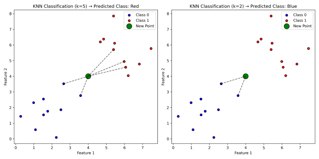
A K that’s too small can cause overfitting, making the model oversensitive to noise. Conversely, a K that’s too large leads to underfitting and loss of important details.
To find the best k value, use the elbow method: plot error rates (or accuracy) against increasing k values. You’ll see that as k increases, the error initially decreases but eventually plateaus. The optimal k value occurs at this “elbow” point—where further increases in k yield minimal improvement in error reduction.
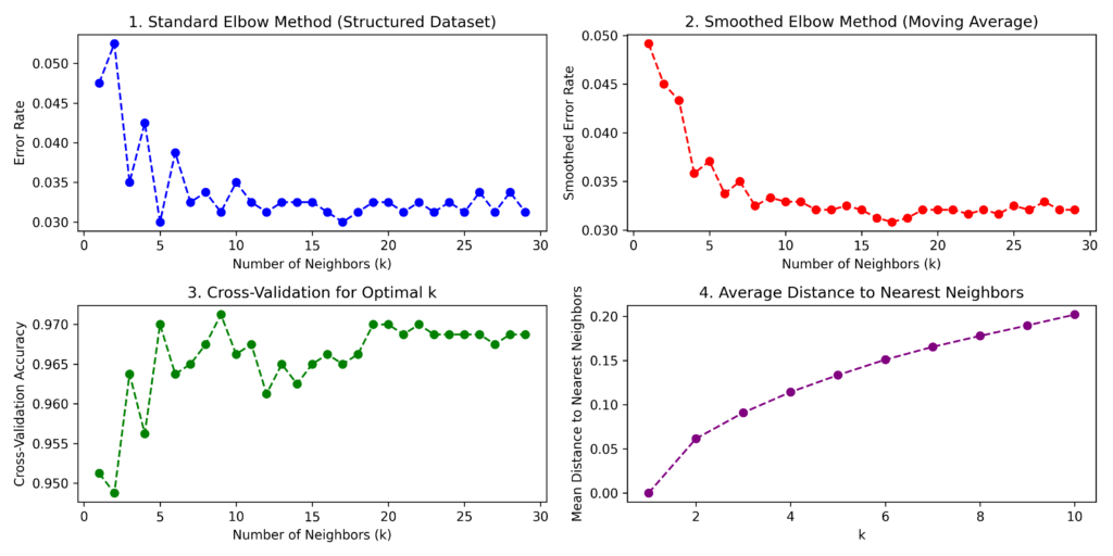
You can also find the optimal K value using grid search or cross-validation techniques.
Model’s performance
The model’s performance is evaluated using these metrics:
- Accuracy: The percentage of correct classifications
from sklearn.metrics import accuracy_score
accuracy = accuracy_score(y_test, y_pred)
print(f'Accuracy: {accuracy:.2f}')- Confusion matrix: A comparison of predicted versus actual classes
from sklearn.metrics import confusion_matrix
import seaborn as sns
import matplotlib.pyplot as plt

conf_matrix = confusion_matrix(y_test, y_pred)
sns.heatmap(conf_matrix, annot=True, fmt='d', cmap='Blues', xticklabels=['No Disease', 'Disease'], yticklabels=['No Disease', 'Disease'])
plt.xlabel('Predicted')
plt.ylabel('Actual')
plt.title('Confusion Matrix')
plt.show()- Classification report: Displays precision, recall, and F1 score metrics
from sklearn.metrics import classification_report
print(classification_report(y_test, y_pred))
Complete Python Program
In this program, we implement all the guidelines discussed above.
We begin by creating a sample patient dataset containing three features: age, systolic blood pressure, and cholesterol values.
Each patient record includes a binary label indicating their health status.
We then divide our dataset into training and test portions.
After standardizing the data values,
we train our model using the prepared dataset.
Next, we assess the model’s effectiveness.
Finally, we create a visualization showing the decision boundary between two selected features.
import numpy as np
import pandas as pd
import matplotlib.pyplot as plt
import seaborn as sns
from sklearn.model_selection import train_test_split
from sklearn.preprocessing import StandardScaler
from sklearn.neighbors import KNeighborsClassifier
from sklearn.metrics import accuracy_score, confusion_matrix, classification_report
from matplotlib.colors import ListedColormap

# Generate synthetic medical dataset
np.random.seed(42)
n_samples = 300

# Features: Age, Blood Pressure, Cholesterol
age = np.random.randint(20, 80, n_samples)
bp = np.random.randint(80, 180, n_samples)
cholesterol = np.random.randint(150, 300, n_samples)

# Target: Disease (0 = No Disease, 1 = Disease)
disease = ((age > 50) & (bp > 130) & (cholesterol > 220)).astype(int)

# Create DataFrame
data = pd.DataFrame({'Age': age, 'Blood Pressure': bp, 'Cholesterol': cholesterol, 'Disease': disease})

# Split dataset
X = data[['Age', 'Blood Pressure', 'Cholesterol']]
y = data['Disease']
X_train, X_test, y_train, y_test = train_test_split(X, y, test_size=0.2, random_state=42)

# Standardize features
scaler = StandardScaler()
X_train_scaled = scaler.fit_transform(X_train)
X_test_scaled = scaler.transform(X_test)

# Train KNN model
knn = KNeighborsClassifier(n_neighbors=5)
knn.fit(X_train_scaled, y_train)

# Predictions
y_pred = knn.predict(X_test_scaled)

# Evaluate performance
accuracy = accuracy_score(y_test, y_pred)
conf_matrix = confusion_matrix(y_test, y_pred)

# Print classification report
print(f'Accuracy: {accuracy:.2f}')
print(classification_report(y_test, y_pred))

# Plot confusion matrix
plt.figure(figsize=(6,4))
sns.heatmap(conf_matrix, annot=True, fmt='d', cmap='Blues', xticklabels=['No Disease', 'Disease'], yticklabels=['No Disease', 'Disease'])
plt.xlabel('Predicted')
plt.ylabel('Actual')
plt.title('Confusion Matrix')
plt.show()

# Decision boundary visualization (2D projection of 3D space)
def plot_decision_boundary(model, X, y):
    X = X[:, [0, 1]]  # Use first two features for visualization
    x_min, x_max = X[:, 0].min() - 1, X[:, 0].max() + 1
    y_min, y_max = X[:, 1].min() - 1, X[:, 1].max() + 1
    xx, yy = np.meshgrid(np.linspace(x_min, x_max, 100), np.linspace(y_min, y_max, 100))
    Z = model.predict(np.c_[xx.ravel(), yy.ravel(), np.zeros(xx.ravel().shape)])  # Adding a zero column to match dimensions
    Z = Z.reshape(xx.shape)

    plt.contourf(xx, yy, Z, alpha=0.3, cmap=ListedColormap(['lightblue', 'lightcoral']))
    scatter = plt.scatter(X[:, 0], X[:, 1], c=y, cmap=ListedColormap(['blue', 'red']), edgecolors='k')
    plt.xlabel('Age')
    plt.ylabel('Blood Pressure')
    plt.title('Decision Boundary')
    plt.legend(handles=scatter.legend_elements()[0], labels=['No Disease', 'Disease'])
    plt.show()

plot_decision_boundary(knn, X_train_scaled, y_train)
Additional Resources
Wikipedia — k-nearest neighbors algorithm – Wikipedia
Python Machine Learning – K-nearest neighbors (KNN)
KNeighborsClassifier — scikit-learn 1.6.1 documentation
Conclusions
KNN is a powerful algorithm for classification tasks, though less effective for regression. Its strengths lie in its simplicity, non-parametric nature (no assumptions about data distribution), and strong performance with small datasets.
However, the algorithm has limitations—it struggles with large datasets containing many features and shows sensitivity to both scale differences and outliers.