Machine Learning Distances - micheledpierri.com: statistics, data analysis and coding

Introduction

Let’s understand Machine Learning Distances through a simple example.

Imagine planning a vacation to a city with an attraction you want to visit. To avoid wasting time traveling, you search for a hotel near this attraction.

But how can you evaluate the distances between several potential hotels to find the closest one?

This typical real-life situation translates well to data analysis. Instead of measuring the distance between hotels and attractions, we want to determine if data points—for example, from two different patients—are similar (close) or dissimilar (far apart).

Many machine learning algorithms are built on methods developed to solve this fundamental question.

Imagine our dataset as a set of points in space, where each observation (or record) represents a single point.

For example, a patient (x) can be described by several features: blood pressure (x₁), cholesterol (x₂), body mass index (x₃), and blood glucose (x₄).

Since we have four features, each patient can be represented by a point in a four-dimensional space.

Patient	Pressure (mmHg)	Cholesterol (mg/dL)	BMI	Blood glucose (mg/dL)
A	140	220	27	100
B	130	190	25	90
C	160	250	30	120

The points can be summarized as follows:

A = (140, 220, 27, 100)

B = (130, 190, 25, 90)

C = (160, 250, 30, 120)

This mathematical space containing these points is called the feature space, where each point is represented as a vector. Depending on the number of features used, the space can have any number of dimensions.

$X = (x_1, x_2, ..., x_n) \in \mathbb{R}^n$

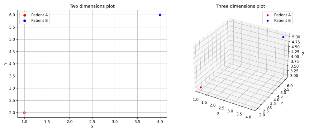
Visualizing the feature space is straightforward in two dimensions, more challenging in three dimensions, and increasingly difficult in higher-dimensional spaces—where our visual capabilities fall short.

Distances between two patients in two and three dimensions

Distance Measurements

Machine learning offers numerous methods for calculating distances between points:

Euclidean Distance

Mahnattan Distance

Minkowski Distance

Hamming Distance

Cosine Distance

Mahalanobis Distance

Jaccard Distance

Bray-Curtis Distance

Hellinger Distance

Let’s explore the most widely used approaches.

Euclidean Distance

Euclidean distance is the simplest way to measure how far apart two points are. In a two-dimensional plane, it’s the length of the straight line that connects them.

This distance measure comes from the Pythagorean theorem, which tells us that in a right triangle, the square of the hypotenuse equals the sum of squares of the other two sides. For two points A and B with coordinates x₁y₁ and x₂y₂, we can apply this theorem:

$d(A, B) = \sqrt{(x_2 - x_1)^2 + (y_2 - y_1)^2}$

We can extend this to calculate the distance between any two points in an n-dimensional space:

$d(X, Y) = \sqrt{\sum_{i=1}^{n} (x_i - y_i)^2}$

To see this in action, let’s look at two patients, A and B. Patient A has a blood pressure of 140 mmHg and cholesterol of 250 mg/dl, while Patient B has values of 130 mmHg and 220 mg/dl respectively.

Here’s how we calculate their Euclidean distance:

$\text{Euclidean Distance} = d(A, B) = \sqrt{(140 - 130)^2 + (250 - 220)^2}$

$= \sqrt{10^2 + 30^2}$

$= \sqrt{100 + 900}$

$= \sqrt{1000} \approx 31.62$

This value of 31.62 tells us how different these patients are: a smaller number means the patients are more similar.

Euclidean distance works best under these conditions:

The features are continuous numbers with similar scales
The dataset has relatively few dimensions. With too many dimensions, Euclidean distance loses effectiveness due to the Curse of Dimensionality—as dimensions increase, the distances between points become more uniform and less meaningful.

Manhattan Distance

Manhattan distance (also known as “city block distance” or “grid distance”) measures the path between points using only vertical and horizontal movements, not diagonal ones. The name comes from Manhattan’s street grid layout in New York City, where streets intersect at right angles.

The Manhattan distance formula is:

$d(X, Y) = \sum_{i=1}^{n} |x_i - y_i|$

This method simply adds up the absolute differences between corresponding points, without squaring them like in Euclidean distance.

Manhattan distance is particularly effective when working with data that naturally follows a grid pattern—such as medical images—or when analyzing categorical data represented by integers.

Minkowski Distance

The Minkowski distance generalizes distance calculations between points into a single formula that can function as either Euclidean or Manhattan distance, depending on the parameter p.

When p equals 1, Minkowski distance acts as Manhattan distance; when p equals 2, it becomes Euclidean distance. Values of p greater than 2 place more emphasis on larger differences between measurements.

The Minkowski distance formula is:

$d(X, Y) = \left( \sum_{i=1}^{n} |x_i - y_i|^p \right)^{\frac{1}{p}}$

By adjusting the parameter p, the Minkowski distance lets us evaluate distances using different methods—making it particularly valuable when we’re uncertain which method will work best.

Hamming Distance

For non-numerical data (like blood types or medications), traditional distance calculations aren’t suitable. The Hamming method offers a solution by counting the differences between features across observations.

Consider two patients’ therapies: Patient A takes Aspirin and Insulin, while Patient B takes Paracetamol and Insulin.

Using the Hamming method, the distance between these patients is 1—representing their single difference in medication.

The Hamming distance formula is as follows:

$d(X, Y) = \sum_{i=1}^{n} \mathbf{1} (x_i \neq y_i)$

This formula effectively compares categorical data or strings (such as DNA sequences).

Cosine Distance

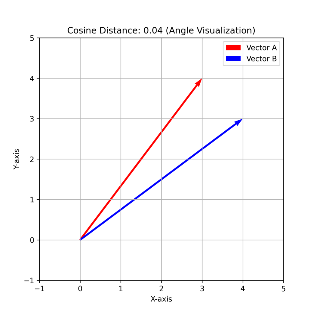
Cosine distance measures the angle between two vectors rather than their absolute difference (magnitude). Since it uses cosine, the result ranges from 0 (identical vectors) to 1 (completely different vectors).

$d_{cos}(X, Y) = 1 - \frac{\sum_{i=1}^{n} x_i y_i}{\sqrt{\sum_{i=1}^{n} x_i^2} \cdot \sqrt{\sum_{i=1}^{n} y_i^2}}$

This distance measure is particularly useful for vector-based features, such as text documents or image data.

Mahalanobis Distance

The Mahalanobis distance measures how far apart points are while accounting for both the correlation between variables and their variance.

$d_M(X, Y) = \sqrt{(X - Y)^T S^{-1} (X - Y)}$

Here, S⁻¹ represents the covariance matrix of the dataset.

This distance measure is particularly useful for datasets with correlated features (such as blood glucose and insulin levels). When features are uncorrelated, it yields results similar to Euclidean distance.

Jaccard Distance

The Jaccard distance measures the dissimilarity between two sets by comparing their shared and unique elements.

$d_J(X, Y) = 1 - \frac{|X \cap Y|}{|X \cup Y|}$

This measure yields values between 0 and 1, where 0 indicates identical sets and 1 indicates completely distinct sets.

In medicine, the Jaccard distance helps analyze symptom patterns for disease prediction and compare DNA sequences.

Bray-Curtis Distance

The Bray-Curtis distance measures the relative difference between two vectors.

$\displaystyle d_{BC}(X, Y) = \frac{\sum_{i=1}^{n} |x_i - y_i|}{\sum_{i=1}^{n} (x_i + y_i)}$

This metric is particularly useful for comparing proportions, such as the ratio between lean mass and body fat, or analyzing differences in bacterial population compositions across samples.

Hellinger Distance

This metric compares probability distributions to measure their similarity.

$d_H(X, Y) = \frac{1}{\sqrt{2}} \sqrt{\sum_{i=1}^{n} (\sqrt{x_i} - \sqrt{y_i})^2}$

It helps analyze differences in marker distributions between healthy and sick subjects and detect bias in medical data.

Summary table

Metric	Data Type	Advantages	Disadvantages
Euclidean	Continuous numbers	Intuitive to understand	Sensitive to scale differences
Manhattan	Grid-based data	Robust against outliers	Less accurate with continuous data
Minkowski	Generalizes Euclidean and Manhattan	Highly flexible	Requires parameter p selection
Cosine	Text, images	Magnitude-independent	Poor performance with zero values
Mahalanobis	Correlated data	Accounts for variance	Requires covariance computation
Jaccard	Sets, binary data	Works well with categories	Ignores difference magnitudes
Bray-Curtis	Compositional data	Handles proportions well	Cannot process negative values
Hellinger	Probability distributions	Ideal for probabilistic data	Needs distribution-formatted data

Python Implementation of Distance Metrics

The script creates a synthetic dataset with medical features (Systolic Pressure, Cholesterol, Glucose, and BMI). It then selects two random patients and calculates various distances between them using Euclidean, Manhattan, Minkowski (p=3), Cosine, Mahalanobis, Jaccard, Bray-Curtis, Hellinger, and Hamming metrics.

import numpy as np
import pandas as pd
import matplotlib.pyplot as plt
import seaborn as sns
from sklearn.preprocessing import MinMaxScaler

def euclidean_distance(x, y):
    return np.sqrt(np.sum((x - y) ** 2))

def manhattan_distance(x, y):
    return np.sum(np.abs(x - y))

def minkowski_distance(x, y, p):
    return np.sum(np.abs(x - y) ** p) ** (1 / p)

def cosine_distance(x, y):
    return 1 - (np.dot(x, y) / (np.linalg.norm(x) * np.linalg.norm(y)))

def mahalanobis_distance(x, y, cov_inv):
    diff = x - y
    return np.sqrt(np.dot(np.dot(diff.T, cov_inv), diff))

def jaccard_distance(x, y):
    intersection = np.sum(np.minimum(x, y))
    union = np.sum(np.maximum(x, y))
    return 1 - intersection / union

def bray_curtis_distance(x, y):
    return np.sum(np.abs(x - y)) / np.sum(x + y)

def hellinger_distance(x, y):
    x = np.array(x, dtype=np.float64)
    y = np.array(y, dtype=np.float64)
    return (1 / np.sqrt(2)) * np.sqrt(np.sum((np.sqrt(x + 1e-10) - np.sqrt(y + 1e-10)) ** 2))

# Generate a synthetic dataset with medical data
np.random.seed(42)
num_patients = 10

data = {
    "Patient": [f"P{i+1}" for i in range(num_patients)],
    "Systolic_Pressure": np.random.randint(100, 180, num_patients),  # mmHg
    "Cholesterol": np.random.randint(150, 250, num_patients),  # mg/dL
    "Glucose": np.random.randint(70, 200, num_patients),  # mg/dL
    "BMI": np.round(np.random.uniform(18, 35, num_patients), 1),  # kg/m^2
    "Smoking": np.random.choice(["Yes", "No"], num_patients),  # Categorical
}

df = pd.DataFrame(data)

# Normalize numerical features to avoid scale imbalances
scaler = MinMaxScaler()
df_scaled = df.copy()
df_scaled.iloc[:, 1:-1] = scaler.fit_transform(df.iloc[:, 1:-1])

# Convert categorical column "Smoking" into numerical for Hamming distance
df_scaled["Smoking"] = df["Smoking"].map({"No": 0, "Yes": 1})

# Compute covariance matrix for Mahalanobis distance
cov_matrix = np.cov(df_scaled.iloc[:, 1:-1].T)
cov_inv = np.linalg.inv(cov_matrix)

# Select two random patients to compute distances
p1, p2 = np.random.choice(df_scaled.index, 2, replace=False)
X_p1 = df_scaled.iloc[p1, 1:].values
X_p2 = df_scaled.iloc[p2, 1:].values

# Compute distances
dist_euclidean = euclidean_distance(X_p1, X_p2)
dist_manhattan = manhattan_distance(X_p1, X_p2)
dist_minkowski_3 = minkowski_distance(X_p1, X_p2, 3)
dist_cosine = cosine_distance(X_p1, X_p2)
dist_mahalanobis = mahalanobis_distance(X_p1[:-1], X_p2[:-1], cov_inv)
dist_jaccard = jaccard_distance(X_p1[:-1], X_p2[:-1])
dist_bray_curtis = bray_curtis_distance(X_p1[:-1], X_p2[:-1])
dist_hellinger = hellinger_distance(X_p1[:-1], X_p2[:-1])
dist_hamming = np.sum(X_p1[:-1] != X_p2[:-1])  # Excluding categorical variable

# Create a results dataframe
dist_results = pd.DataFrame({
    "Distance": ["Euclidean", "Manhattan", "Minkowski (p=3)", "Cosine", "Mahalanobis", "Jaccard", "Bray-Curtis", "Hellinger", "Hamming"],
    "Value": [dist_euclidean, dist_manhattan, dist_minkowski_3, dist_cosine, dist_mahalanobis, dist_jaccard, dist_bray_curtis, dist_hellinger, dist_hamming]
})

# Plot the distance comparison
fig, ax = plt.subplots(figsize=(10, 6))
sns.barplot(x=dist_results["Distance"], y=dist_results["Value"], ax=ax, palette="coolwarm")
ax.set_title("Comparison of Different Distance Metrics", fontsize=14)
ax.set_ylabel("Distance Value", fontsize=12)
ax.set_xlabel("Distance Type", fontsize=12)
ax.grid(axis="y", linestyle="--", alpha=0.7)
ax.set_xticklabels(ax.get_xticklabels(), rotation=45, ha="right")

# Annotate bars with values
for i, v in enumerate(dist_results["Value"]):
    ax.text(i, v + 0.05, f"{v:.2f}", ha='center', fontsize=12)

plt.show()

import numpy as np
import pandas as pd
import matplotlib.pyplot as plt
import seaborn as sns
from sklearn.preprocessing import MinMaxScaler

def euclidean_distance(x, y):
    return np.sqrt(np.sum((x - y) ** 2))

def manhattan_distance(x, y):
    return np.sum(np.abs(x - y))

def minkowski_distance(x, y, p):
    return np.sum(np.abs(x - y) ** p) ** (1 / p)

def cosine_distance(x, y):
    return 1 - (np.dot(x, y) / (np.linalg.norm(x) * np.linalg.norm(y)))

def mahalanobis_distance(x, y, cov_inv):
    diff = x - y
    return np.sqrt(np.dot(np.dot(diff.T, cov_inv), diff))

def jaccard_distance(x, y):
    intersection = np.sum(np.minimum(x, y))
    union = np.sum(np.maximum(x, y))
    return 1 - intersection / union

def bray_curtis_distance(x, y):
    return np.sum(np.abs(x - y)) / np.sum(x + y)

def hellinger_distance(x, y):
    x = np.array(x, dtype=np.float64)
    y = np.array(y, dtype=np.float64)
    return (1 / np.sqrt(2)) * np.sqrt(np.sum((np.sqrt(x + 1e-10) - np.sqrt(y + 1e-10)) ** 2))

# Generate a synthetic dataset with medical data
np.random.seed(42)
num_patients = 10

data = {
    "Patient": [f"P{i+1}" for i in range(num_patients)],
    "Systolic_Pressure": np.random.randint(100, 180, num_patients),  # mmHg
    "Cholesterol": np.random.randint(150, 250, num_patients),  # mg/dL
    "Glucose": np.random.randint(70, 200, num_patients),  # mg/dL
    "BMI": np.round(np.random.uniform(18, 35, num_patients), 1),  # kg/m^2
    "Smoking": np.random.choice(["Yes", "No"], num_patients),  # Categorical
}

df = pd.DataFrame(data)

# Normalize numerical features to avoid scale imbalances
scaler = MinMaxScaler()
df_scaled = df.copy()
df_scaled.iloc[:, 1:-1] = scaler.fit_transform(df.iloc[:, 1:-1])

# Convert categorical column "Smoking" into numerical for Hamming distance
df_scaled["Smoking"] = df["Smoking"].map({"No": 0, "Yes": 1})

# Compute covariance matrix for Mahalanobis distance
cov_matrix = np.cov(df_scaled.iloc[:, 1:-1].T)
cov_inv = np.linalg.inv(cov_matrix)

# Select two random patients to compute distances
p1, p2 = np.random.choice(df_scaled.index, 2, replace=False)
X_p1 = df_scaled.iloc[p1, 1:].values
X_p2 = df_scaled.iloc[p2, 1:].values

# Compute distances
dist_euclidean = euclidean_distance(X_p1, X_p2)
dist_manhattan = manhattan_distance(X_p1, X_p2)
dist_minkowski_3 = minkowski_distance(X_p1, X_p2, 3)
dist_cosine = cosine_distance(X_p1, X_p2)
dist_mahalanobis = mahalanobis_distance(X_p1[:-1], X_p2[:-1], cov_inv)
dist_jaccard = jaccard_distance(X_p1[:-1], X_p2[:-1])
dist_bray_curtis = bray_curtis_distance(X_p1[:-1], X_p2[:-1])
dist_hellinger = hellinger_distance(X_p1[:-1], X_p2[:-1])
dist_hamming = np.sum(X_p1[:-1] != X_p2[:-1])  # Excluding categorical variable

# Create a results dataframe
dist_results = pd.DataFrame({
    "Distance": ["Euclidean", "Manhattan", "Minkowski (p=3)", "Cosine", "Mahalanobis", "Jaccard", "Bray-Curtis", "Hellinger", "Hamming"],
    "Value": [dist_euclidean, dist_manhattan, dist_minkowski_3, dist_cosine, dist_mahalanobis, dist_jaccard, dist_bray_curtis, dist_hellinger, dist_hamming]
})

# Plot the distance comparison
fig, ax = plt.subplots(figsize=(10, 6))
sns.barplot(x=dist_results["Distance"], y=dist_results["Value"], ax=ax, palette="coolwarm")
ax.set_title("Comparison of Different Distance Metrics", fontsize=14)
ax.set_ylabel("Distance Value", fontsize=12)
ax.set_xlabel("Distance Type", fontsize=12)
ax.grid(axis="y", linestyle="--", alpha=0.7)
ax.set_xticklabels(ax.get_xticklabels(), rotation=45, ha="right")

# Annotate bars with values
for i, v in enumerate(dist_results["Value"]):
    ax.text(i, v + 0.05, f"{v:.2f}", ha='center', fontsize=12)

plt.show()

Bar comparison of different distance metrics

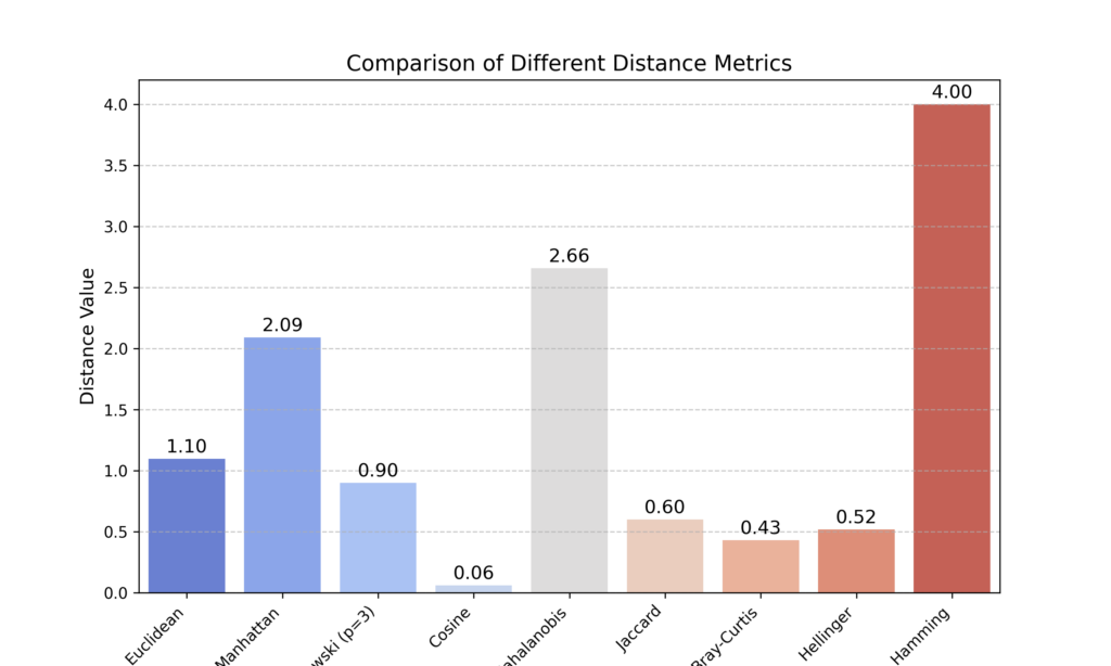
While the results are plotted to compare these distance metrics, it’s important to note that each metric serves a specific purpose based on the dataset’s characteristics.

However, the resulting graph is potentially misleading since each metric uses different formulas and has distinct interpretations that must be considered in context.

For example, the Cosine, Jaccard, Bray-Curtis, and Hellinger methods have values that range between 0 and 1, while other methods can have any value.

Additional Resources

Juan Luis Suárez, Salvador García, Francisco Herrera, A tutorial on distance metric learning: Mathematical foundations, algorithms, experimental analysis, prospects and challenges, Neurocomputing, Volume 425, 2021, Pages 300-322, ISSN 0925-2312

Metric Learning

Kaggle. Distance measures in machine learning

Conclusions

Selecting the right distance metric is crucial for successful machine learning analysis. Rather than having one “best” metric, different metrics suit different types of data and goals:

Euclidean distance works best for continuous numerical data in low-dimensional spaces
Manhattan distance suits data organized in grid-like structures
Mahalanobis distance excels when working with correlated variables
Hamming or Jaccard distances are ideal for categorical or binary data

Keep in mind the computational costs: some metrics, such as Mahalanobis, involve complex calculations that may be impractical for large datasets.

Before choosing a distance metric, consider these key factors:

The type of data you’re working with (numerical, categorical, or mixed)
Whether your variables are correlated
The number of dimensions in your feature space
Whether your data needs normalization to ensure fair comparisons

In practice, it’s often valuable to experiment with different distance metrics and determine which one yields the most meaningful results for your specific problem.