
Introduction: Why Evaluation Deserves More Attention Than Modelling
In daily practice, most of the time spent on a machine learning project goes into building models. Evaluation, paradoxically, is often the rushed phase. Yet without the right metric, a clever algorithm and a coin flip can look surprisingly similar on paper.
This guide walks through the metrics that actually matter, when each is appropriate, and how to compute them in Python. The angle is unapologetically applied: examples are kept short, the framing is borrowed from clinical research where possible, and pitfalls are flagged where they have caused real problems in published work.
A small disclaimer up front. No single metric tells the whole story. The number you choose to report is, in effect, a small editorial decision about what kinds of error you are willing to tolerate.
Classification Models: When the Target is a Category
Confusion Matrix: The Foundation
- Formal definition: for binary classification, the confusion matrix M ∈ R^{2×2} has entries M_{ij} equal to the number of examples with true class i predicted as class j. By convention the four cells are TN, FP, FN, TP.
- Intuition: every other classification metric is a summary of these four counts. Always look at the matrix first, especially when classes are imbalanced. In an unbalanced clinical dataset, a model that predicts “no event” for everyone can score well on accuracy and still be useless.

Accuracy: Simple, Sometimes Misleading
- Formal definition: Accuracy = (TP + TN) / (TP + TN + FP + FN).
- Intuition: the fraction of correct predictions. It works reasonably well with balanced classes. Under heavy imbalance (think operative mortality at 2%, or a rare arrhythmia), it tends to flatter the model.
accuracy = (TP + TN) / (TP + TN + FP + FN)
Precision vs Recall: The Trade-off That Matters
- Formal definitions:
- Precision = TP / (TP + FP)
- Recall (also Sensitivity, TPR) = TP / (TP + FN)
- Intuition. Precision answers the question “of the cases I flagged as positive, how many really were?” It is the metric that controls false alarms. Recall answers the complementary question, “of the truly positive cases, how many did I catch?” It is the metric that controls misses.
In a triage setting, recall almost always wins. In a screening pathway that triggers an invasive procedure, precision becomes the constraint. The two rarely move together.
from sklearn.metrics import precision_score, recall_score

y_true = [0, 1, 1, 0, 1, 0, 1, 1]
y_pred = [0, 1, 0, 0, 1, 0, 1, 1]

precision = precision_score(y_true, y_pred)
recall = recall_score(y_true, y_pred)
print(f"Precision: {precision:.2f} | Recall: {recall:.2f}")
F1-Score: A Single Number When Both Errors Count
- Formal definition: F1 = 2 · (Precision · Recall) / (Precision + Recall).
- Intuition: the harmonic mean of precision and recall. It collapses to a low value if either component is low, which makes it a sensible summary when both kinds of error matter and the classes are imbalanced.
from sklearn.metrics import f1_score

f1 = f1_score(y_true, y_pred, average='weighted')
print(f"F1-Score: {f1:.2f}")
ROC-AUC and PR-AUC: Threshold-Independent Ranking
- Formal definitions:
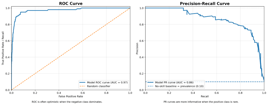
- ROC curve: a plot of TPR against FPR as the decision threshold sweeps through its range. AUC_ROC = ∫ TPR d(FPR).
- PR curve: a plot of Precision against Recall. Average Precision (AP) is the area under the PR curve, computed as a step-wise average of precision at the unique recall levels.
- Intuition. ROC-AUC measures the model’s overall ability to rank positive cases above negative ones. With strong class imbalance (the typical clinical case), PR-AUC and AP capture early-recall behaviour better, which is what matters when the operating point lives at a low false-positive rate.
from sklearn.metrics import roc_auc_score, average_precision_score, PrecisionRecallDisplay
import numpy as np

y_scores = np.array([0.1, 0.8, 0.4, 0.2, 0.9, 0.3, 0.85, 0.7])
y_true = np.array([0, 1, 1, 0, 1, 0, 1, 1])

roc_auc = roc_auc_score(y_true, y_scores)
ap = average_precision_score(y_true, y_scores)
print(f"ROC-AUC: {roc_auc:.3f} | PR-AUC (AP): {ap:.3f}")

PrecisionRecallDisplay.from_predictions(y_true, y_scores)
Calibration: Are the Probabilities Trustworthy?
- Formal definitions:
- Brier score = (1/N) ∑ (p_i − y_i)^2
- Log loss = −(1/N) ∑ [ y_i log p_i + (1 − y_i) log (1 − p_i) ]
- Intuition. A model can have an excellent AUC and still produce probabilities that nobody should trust. The reason is simple: AUC measures ranking, not calibration. Reliability diagrams together with Brier or LogLoss tell you whether a predicted “20% risk” really behaves like one in five. When the answer is no, Platt (sigmoid) or isotonic post-hoc calibration are the usual remedies.
from sklearn.calibration import calibration_curve
from sklearn.metrics import brier_score_loss, log_loss

brier = brier_score_loss(y_true, y_scores)
ll = log_loss(y_true, y_scores)
print(f"Brier: {brier:.4f} | LogLoss: {ll:.4f}")

prob_true, prob_pred = calibration_curve(y_true, y_scores, n_bins=10, strategy='quantile')
Calibration pitfalls
- Never calibrate and evaluate on the same data; use cross-validation or a held-out set.
- Isotonic calibration tends to overfit when the sample is small. Sigmoid (Platt) is more stable in low-data regimes.
- Calibration drifts. Monitor it over time and be ready to recalibrate.
- Calibrate raw probabilities, not hard-thresholded scores.
- With heavy imbalance, quantile binning produces more honest reliability diagrams than equal-width bins. </aside>

Threshold Tuning with Fβ
- Formal definition: Fβ = (1 + β²) · (P · R) / (β² · P + R).
- Intuition: β > 1 prioritises recall, β < 1 prioritises precision. Pick the probability threshold that maximises Fβ for the chosen β. In the clinic, the choice of β is essentially a decision about the relative cost of a missed case versus a false alarm. It is rarely made consciously, which is part of the problem.
import numpy as np
from sklearn.metrics import precision_recall_curve

# Given y_true (0/1) and y_scores (probabilities)
prec, rec, th = precision_recall_curve(y_true, y_scores)
beta = 2.0  # prioritise recall (F2)
eps = 1e-12
f_beta = (1 + beta**2) * (prec * rec) / (beta**2 * prec + rec + eps)
# align with thresholds (len(prec) = len(th)+1)
best_idx = int(np.nanargmax(f_beta[1:]))
best_threshold = float(th[best_idx])
print(f"Best threshold for F{beta:.0f}: {best_threshold:.3f} | F{beta:.0f}_max: {np.nanmax(f_beta):.3f}")

# use the tuned threshold
y_pred_tuned = (y_scores >= best_threshold).astype(int)

CalibratedClassifierCV: Platt (sigmoid) vs Isotonic
- Intuition: compare the two methods with cross-validation. The one with the lower Brier or LogLoss, and the better-looking reliability curve, wins. They rarely tie.
from sklearn.model_selection import train_test_split
from sklearn.linear_model import LogisticRegression
from sklearn.calibration import CalibratedClassifierCV
from sklearn.metrics import brier_score_loss, log_loss

# Suppose you already have X (features) and y (0/1 labels)
X_train, X_val, y_train, y_val = train_test_split(
    X, y, test_size=0.2, random_state=42, stratify=y
)

base = LogisticRegression(max_iter=1000, class_weight='balanced', random_state=42)
base.fit(X_train, y_train)
y_val_base = base.predict_proba(X_val)[:, 1]
print("Base   ", "Brier:", brier_score_loss(y_val, y_val_base),
      "LogLoss:", log_loss(y_val, y_val_base))

# Platt scaling (sigmoid)
platt = CalibratedClassifierCV(base_estimator=base, method='sigmoid', cv=5)
platt.fit(X_train, y_train)
y_val_platt = platt.predict_proba(X_val)[:, 1]
print("Platt  ", "Brier:", brier_score_loss(y_val, y_val_platt),
      "LogLoss:", log_loss(y_val, y_val_platt))

# Isotonic regression (more flexible)
isot = CalibratedClassifierCV(base_estimator=base, method='isotonic', cv=5)
isot.fit(X_train, y_train)
y_val_isot = isot.predict_proba(X_val)[:, 1]
print("Isot   ", "Brier:", brier_score_loss(y_val, y_val_isot),
      "LogLoss:", log_loss(y_val, y_val_isot))

# Pick the best calibrated scores (here, by Brier)
y_scores = (
    y_val_isot
    if brier_score_loss(y_val, y_val_isot) < brier_score_loss(y_val, y_val_platt)
    else y_val_platt
)
Beyond Accuracy and F1: Balanced Accuracy, MCC, Cohen’s Kappa
- Formal definitions:
- Balanced Accuracy = (TPR + TNR) / 2
- MCC = (TP·TN − FP·FN) / sqrt((TP+FP)(TP+FN)(TN+FP)(TN+FN))
- Cohen’s κ = (p_o − p_e) / (1 − p_e), with p_o the observed agreement and p_e the agreement expected by chance.
- Intuition. Balanced accuracy is more honest than plain accuracy when the classes are skewed. MCC is, in practice, the most informative single number for very imbalanced binary problems; it stays sensible even when one cell of the confusion matrix is empty. Cohen’s κ has a different flavour: it measures agreement above chance and is the natural choice when comparing a model against human raters, or two raters against each other.
from sklearn.metrics import balanced_accuracy_score, matthews_corrcoef, cohen_kappa_score

bal_acc = balanced_accuracy_score(y_true, y_pred)
mcc = matthews_corrcoef(y_true, y_pred)
kappa = cohen_kappa_score(y_true, y_pred)
print(f"Balanced Acc: {bal_acc:.3f} | MCC: {mcc:.3f} | Kappa: {kappa:.3f}")
Statistical Tests: McNemar and AUC Confidence Intervals
- Formal definitions:
- McNemar’s test evaluates the null hypothesis that two classifiers have equal error rates on paired predictions.
- AUC variance is typically estimated via DeLong’s method or by bootstrap, which yields confidence intervals and a basis for comparison.
- Intuition: small differences in metric values are not always meaningful. Quantifying the uncertainty is the part that turns a comparison into a claim. In small clinical samples, this step is non-negotiable.
from statsmodels.stats.contingency_tables import mcnemar
import numpy as np

# b = A wrong, B right; c = A right, B wrong
b = np.sum((y_pred_A != y_true) & (y_pred_B == y_true))
c = np.sum((y_pred_A == y_true) & (y_pred_B != y_true))
res = mcnemar([[0, b], [c, 0]], exact=False, correction=True)
print(f"McNemar chi2={res.statistic:.3f}, p={res.pvalue:.4f}")
from sklearn.metrics import roc_auc_score
import numpy as np
rng = np.random.default_rng(42)

def auc_bootstrap_ci(y, p, B=2000, alpha=0.05):
    aucs = []
    n = len(y)
    for _ in range(B):
        idx = rng.integers(0, n, n)
        aucs.append(roc_auc_score(y[idx], p[idx]))
    lo, hi = np.percentile(aucs, [100 * alpha / 2, 100 * (1 - alpha / 2)])
    return float(np.mean(aucs)), float(lo), float(hi)

auc_mean, lo, hi = auc_bootstrap_ci(y_true, y_scores)
print(f"AUC bootstrap mean={auc_mean:.3f} | 95% CI [{lo:.3f}, {hi:.3f}]")
Regression Models: When the Target is a Number
MAE and MSE: Measuring Error Magnitude
- Formal definitions:
- MAE = (1/N) ∑ |y_i − ŷ_i|
- MSE = (1/N) ∑ (y_i − ŷ_i)^2, with RMSE = √MSE.
- Intuition. MAE is robust and easy to explain to a non-technical audience. MSE and RMSE penalise large errors disproportionately, which is the right behaviour when a single bad prediction is much more costly than several small ones. It is worth choosing between them deliberately, not by habit.
from sklearn.metrics import mean_absolute_error, mean_squared_error
import numpy as np

# example
y_true = np.array([3.0, 4.5, 2.0, 6.0, 3.5])
y_pred = np.array([2.8, 4.7, 2.1, 5.9, 3.4])

mae = mean_absolute_error(y_true, y_pred)
mse = mean_squared_error(y_true, y_pred)
rmse = np.sqrt(mse)
print(f"MAE={mae:.3f} | MSE={mse:.3f} | RMSE={rmse:.3f}")
R² Score: Explained Variance
- Formal definition: R² = 1 − SS_res / SS_tot = 1 − ∑(y − ŷ)^2 / ∑(y − ȳ)^2.
- Intuition: the fraction of variance explained relative to a constant-mean baseline. R² can in fact be negative; this happens when the model performs worse than simply predicting the mean. A negative R² on a held-out set is a useful warning sign and not, as sometimes assumed, a bug.
from sklearn.metrics import r2_score
import numpy as np

# example
y_true = np.array([300, 450, 200, 600, 350])
y_pred = np.array([280, 470, 210, 590, 340])

r2 = r2_score(y_true, y_pred)
print(f"R² Score: {r2:.3f}")
MAPE: Percentage Error
- Formal definition: MAPE = (100/N) ∑ |(y_i − ŷ_i) / y_i|.
- Intuition: easy to communicate as a percentage. MAPE breaks down (or misleads) when y can take values close to zero, since small denominators inflate the error. In that case, symmetric MAPE or absolute error are safer choices.
import numpy as np
mape = np.mean(np.abs((y_true - y_pred) / y_true)) * 100
print(f"MAPE: {mape:.2f}%")
Clustering Models: The Harder Problem of Unsupervised Evaluation
Silhouette Score: Cohesion vs Separation
- Formal definition: for point i, s_i = (b_i − a_i) / max(a_i, b_i), where a_i is the mean intra-cluster distance for i and b_i the minimum mean distance from i to any other cluster. The overall score is the mean of s_i, in the range [−1, 1].
- Intuition: higher is better. A score near zero suggests overlapping clusters; a negative score points to misassignment. As a single number it is convenient, but rarely sufficient on its own. In phenotyping work, cluster validity is almost always judged jointly with clinical plausibility.
from sklearn.metrics import silhouette_score
from sklearn.cluster import KMeans
import numpy as np

# synthetic example
X = np.random.rand(100, 3)

kmeans = KMeans(n_clusters=4, n_init=10, random_state=42)
labels = kmeans.fit_predict(X)
score = silhouette_score(X, labels)
print(f"Silhouette score: {score:.3f}")
Python Implementation: End-to-End Code Examples
A Full Classification Pipeline
from sklearn.model_selection import train_test_split
from sklearn.ensemble import RandomForestClassifier
from sklearn.metrics import classification_report, confusion_matrix, roc_auc_score
import pandas as pd

# Load dataset (example: Titanic survival)
df = pd.read_csv('titanic.csv')
X = df[['age', 'fare', 'pclass', 'sibsp']]
y = df['survived']

# Split data
X_train, X_test, y_train, y_test = train_test_split(X, y, test_size=0.2, random_state=42)

# Train model
model = RandomForestClassifier(n_estimators=100, random_state=42)
model.fit(X_train, y_train)

# Predictions
y_pred = model.predict(X_test)
y_proba = model.predict_proba(X_test)[:, 1]

print("=== CLASSIFICATION REPORT ===")
print(classification_report(y_test, y_pred, target_names=['Died', 'Survived']))

print("\\n=== CONFUSION MATRIX ===")
print(confusion_matrix(y_test, y_pred))

print("\\n=== ROC-AUC ===")
auc = roc_auc_score(y_test, y_proba)
print(f"ROC-AUC: {auc:.3f}")
A Full Regression Pipeline
from sklearn.model_selection import train_test_split
from sklearn.ensemble import GradientBoostingRegressor
from sklearn.metrics import mean_absolute_error, mean_squared_error, r2_score
import numpy as np
import pandas as pd

# Dataset: predict car prices
df = pd.read_csv('car_prices.csv')
X = df[['mileage', 'year', 'engine_size']]
y = df['price']

# Split and train
X_train, X_test, y_train, y_test = train_test_split(X, y, test_size=0.2, random_state=42)
model = GradientBoostingRegressor(random_state=42)
model.fit(X_train, y_train)

# Predict and evaluate
y_pred = model.predict(X_test)

mae = mean_absolute_error(y_test, y_pred)
rmse = np.sqrt(mean_squared_error(y_test, y_pred))
r2 = r2_score(y_test, y_pred)
mape = np.mean(np.abs((y_test - y_pred) / y_test)) * 100

print(f"MAE: ${mae:,.2f}")
print(f"RMSE: ${rmse:,.2f}")
print(f"R² Score: {r2:.3f}")
print(f"MAPE: {mape:.2f}%")
Choosing the Right Metric: A Decision Framework
| Scenario | Recommended Metric | Why |
|---|---|---|
| Balanced classification | Accuracy plus F1-Score | Simple and robust together |
| Imbalanced classification (e.g. fraud) | Precision/Recall plus PR-AUC (with ROC-AUC for context) | Focus on the minority class and on early-recall behaviour |
| Medical diagnosis | Recall (to be maximised), with calibrated probabilities | False negatives carry the highest clinical cost |
| Spam detection | Precision (to be maximised) | False positives are disruptive to the end user |
| Business forecasting | MAE plus MAPE | Both are interpretable to non-technical stakeholders |
| Scientific modelling | R² plus RMSE | Standard pairing in the literature |
| Customer segmentation | Silhouette plus a business KPI | Internal validity together with downstream usefulness |
Clinical Scenarios: Recommended Metrics
In the clinical setting, metric choice is essentially a statement about which type of error is acceptable. The following table summarises the recommended primary and secondary metrics for the most common scenarios encountered in cardiovascular and perioperative practice.
| Scenario | Primary metrics | Secondary metrics | Rationale | Notes |
|---|---|---|---|---|
| Diagnosis (rule-out of serious disease) | Recall/Sensitivity, NPV | PR-AUC, Fβ (β > 1), ROC-AUC | Missing a true case carries the highest cost; the priority is to catch positives. | Use calibrated probabilities. Cost-sensitive threshold tuning to maximise Fβ with β > 1 is the natural operational lever. |
| Diagnosis (rule-in before invasive therapy) | Precision/PPV, Specificity | ROC-AUC, MCC | False positives lead to unnecessary, sometimes harmful interventions. | Set a higher decision threshold; report LR+ and decision curves where applicable. |
| Triage (ED or ICU prioritisation) | Recall at fixed Precision, early-recall PR curve | Fβ (β ≈ 2), PR-AUC, MCC | Safety first under resource constraints; high capture of critical cases is essential. | Report performance at the operational cutoffs actually in use. Monitor drift, recalibrate regularly. |
| Screening (low prevalence) | PR-AUC (AP), Recall, PPV | ROC-AUC, NNS (1/PPV) | Class imbalance makes PR metrics more informative than ROC. | Calibrate. Communicate the expected number of positives per 1,000 screened at the chosen threshold. |
| Prognosis (risk prediction) | Calibration (Brier, LogLoss) and calibration plot | Discrimination (ROC-AUC), Decision Curve Analysis | Treatment decisions depend on accurate absolute risk, not on ranking alone. | Assess net benefit across plausible thresholds; recalibrate when populations shift. |
| Monitoring models in production | Calibration drift (Brier trend), Recall at threshold | Precision at threshold, alert rate, PSI | The goal is to maintain both safety and a sustainable alert burden as the data shift. | Set alarms on metric bands; periodic threshold re-optimisation. |
A practical caveat. In most cardiac surgery cohorts, prevalence of the outcome of interest (operative mortality, major morbidity, postoperative AKI) is low. ROC-AUC alone tends to look reassuringly high in such datasets even when the model is, for clinical purposes, indistinguishable from EuroSCORE-II at the threshold actually used at the bedside. Reporting calibration and decision-curve analysis alongside discrimination metrics is, in our experience, what separates a paper that survives peer review from one that does not.
Conclusion and Next Steps
A few things are worth taking away from all of this. First, the choice of metric is a clinical or business decision before it is a statistical one. Start from the question, then pick the number. Second, no single metric is enough. A short dashboard of complementary scores is almost always more informative than any one of them on its own. Third, plots still beat numbers when it comes to spotting trouble; confusion matrices, ROC and PR curves, and reliability diagrams reveal patterns that a single summary can hide.
A practical action plan, then:
- Audit current models. Are the metrics in use actually aligned with the decision they support?
- Build a small evaluation template, anchored on the code above, and reuse it across projects.
- Standardise reporting. The same set of metrics, the same plots, the same thresholds.
If you want to turn this into a repeatable workflow, the recipe is short: define the decision goal, pick primary and secondary metrics, choose the operating thresholds, validate calibration, and report uncertainty. Boring, but it works.
See also on this site: Calibration of Predictive Risk Models: A Guide for Clinicians