
Introduction to Random Forest
Random Forests are supervised learning algorithms that belong to the ensemble models. They can be used for both classification and regression. They are based on decision trees.
How Random Forests Work
Random Forests are constructed from multiple decision trees trained on subsets of the original data through a technique called bagging.
Initially, bagging is performed on the original dataset. This involves extracting a random sample of data from the dataset (typically 63% of the data), while the remaining portion forms a validation system called OOB (Out Of Bag).
Each subset of data generated this way is used to train a decision tree, using a random subset of features to split the branches.
For classification problems, the final prediction is determined by the class that receives the majority of votes among all trees.
For regression problems, the final prediction is calculated as the average of all individual tree predictions.
To clarify these steps, let’s examine a simple numerical example with a dataset of 10 observations and three features (x1, x2, x3). The target is the Class column, which can be either 0 or 1:
| Id | X1 | X2 | X3 | Class |
|---|---|---|---|---|
| 1 | 5 | 3 | 1 | 🟢 (0) |
| 2 | 6 | 2 | 2 | 🔴 (1) |
| 3 | 7 | 4 | 3 | 🔴 (1) |
| 4 | 5 | 5 | 2 | 🟢 (0) |
| 5 | 6 | 3 | 3 | 🔴 (1) |
| 6 | 4 | 2 | 1 | 🟢 (0) |
| 7 | 8 | 5 | 3 | 🔴 (1) |
| 8 | 7 | 3 | 2 | 🔴 (1) |
| 9 | 5 | 4 | 1 | 🟢 (0) |
| 10 | 6 | 5 | 2 | 🟢 (0) |
The goal of the Random Forest algorithm is to predict membership in class 0 or 1 based on the three variables.
We proceed with the Bagging technique by dividing the dataset into 3 completely random subsets. The sampling is done with replacement, meaning that after a row is extracted to form a subgroup, it remains in the original dataset and can be selected again for another subgroup. In the examples of subsets that follow, you’ll notice repeated rows (IDs):
| Tree #1 | Tree #2 | Tree #3 |
|---|---|---|
| ID: 1, 2, 3, 7, 8 | ID: 2, 4, 5, 7, 9 | ID: 1, 2, 6, 7, 10 |
In creating subsets, not only is a selection of observations (rows) performed but also of columns (features) to create the greatest possible diversity. The formula commonly used to determine the number of features to randomly select is √p, where p is the total number of features. In this case, with 3 features, it would be approximately √3 ≈ 1.73, which rounds to 2.
For each subset, we create a Decision Tree. For example, with Tree #1, we begin at the root by splitting on X1, then use X2 for the internal node, and continue this process.
After building the trees, we combine the predictions of each tree. For classification, majority voting (hard coding) is used, so if 2 out of 3 predictions are equal to (1), the final class will be (1).
Training Results:
| Observation | Tree #1 | Tree #2 | Tree #3 | Final Prediction |
| ID = 2 | 🟢 (0) | 🔴 (1) | 🔴 (1) | 🔴 (1) → Majority |
| ID = 7 | 🟢 (0) | 🟢 (0) | 🔴 (1) | 🟢 (0) → Majority |
When we apply the model to test data, we might obtain results like the following, which we will subsequently evaluate using various metrics to assess the model’s performance.
| Observation | Tree #1 | Tree #2 | Tree #3 | Final Prediction |
| ID = 11 | 🟢 (0) | 🔴 (1) | 🔴 (1) | 🔴 (1) → Majority |
| ID = 12 | 🔴 (1) | 🟢 (0) | 🟢 (0) | 🟢 (0) → Majority |
| ID = 13 | 🔴 (1) | 🔴 (1) | 🔴 (1) | 🔴 (1) → Majority |
Medical Applications of Random Forest
Random Forest is valued for its ability to handle complex and high-dimensional data, providing robust results.
Published research demonstrates its applications in both clinical settings and medical image analysis, as well as in evaluating laboratory signals and data. From a management perspective, Random Forest has also proven effective in forecasting essential medication demand.
Below are some bibliographic references:
Hong W, Lu Y, Zhou X, Jin S, Pan J, Lin Q, Yang S, Basharat Z, Zippi M, Goyal H. Usefulness of Random Forest Algorithm in Predicting Severe Acute Pancreatitis. Front Cell Infect Microbiol. 2022 Jun 10;12:893294. doi: 10.3389/fcimb.2022.893294IF: 4.6 Q1 . PMID: 35755843; PMCID: PMC9226542.
Loef, B., Wong, A., Janssen, N.A.H. et al. Using random forest to identify longitudinal predictors of health in a 30-year cohort study. Sci Rep 12, 10372 (2022). https://doi.org/10.1038/s41598-022-14632-w
Maturo F, Verde R. Pooling random forest and functional data analysis for biomedical signals supervised classification: Theory and application to electrocardiogram data. Stat Med. 2022 May 30;41(12):2247-2275. doi: 10.1002/sim.9353IF: 1.8 Q1 . Epub 2022 Feb 20. PMID: 35184323; PMCID: PMC9303904.
Pirneskoski J, Tamminen J, Kallonen A, Nurmi J, Kuisma M, Olkkola KT, Hoppu S. Random forest machine learning method outperforms prehospital National Early Warning Score for predicting one-day mortality: A retrospective study. Resusc Plus. 2020 Dec 5;4:100046. doi: 10.1016/j.resplu.2020.100046. PMID: 34223321; PMCID: PMC8244434.
When to Use Random Forest
Random Forest is particularly effective for datasets with numerous features and complex non-linear relationships.
It mitigates overfitting through its multiple-tree structure. Since predictions are determined by majority voting, the algorithm also naturally reduces the influence of outliers.
It handles mixed feature types (numerical and categorical) efficiently without requiring extensive data transformations.
Limitations of using Random Forest
First of all, the model should be avoided when result interpretability is necessary, as it functions essentially as a black box. Despite providing feature importance metrics, the underlying decision-making process remains opaque compared to simpler models like linear regression or individual decision trees, making it challenging to explain specific predictions to stakeholders or regulatory bodies.
Additionally, its computational complexity makes it unsuitable when results are needed quickly or in real-time. The process of constructing multiple decision trees and aggregating their predictions demands substantial processing power and memory resources. Computational costs can also be prohibitively high when working with datasets containing numerous observations and/or features, potentially requiring specialized hardware or cloud computing solutions for efficient execution. This computational burden becomes especially problematic in time-sensitive applications where rapid decision-making is crucial.
Implementing Random Forest in Python
To implement Random Forest in Python, you need the Scikit-learn library, specifically its ensemble module.
Scikit-learn offers four main Random Forest implementations:
- RandomForestClassifier: for classification tasks
- ExtraTreesClassifier: similar to RandomForestClassifier but faster and with increased randomization
- RandomForestRegressor: for regression problems
- ExtraTreesRegressor: similar to RandomForestRegressor but faster and with increased randomization
Random Forest Hyperparameters
When instantiating a Random Forest class, we can specify hyperparameters to customize our model’s behavior.
There are several hyperparameters available. The main ones include:
- Number of trees in the forest: n_estimators (default = 100)
- Depth of trees: max_depth (default = None). This determines the number of branch divisions. If set to None, divisions continue until each leaf contains fewer samples than min_samples_split.
- Number of features to include in each split: max_features. The default “sqrt” uses the square root of the total number of features.
- Minimum number of samples required for a node: min_samples_split. The default value is 2.
- Minimum number of samples per leaf: min_samples_leaf. The default value is 1.
- Sample weighting: applies only to RandomForestClassifier and helps balance uneven class distributions. The default is None, but it can be set to “balanced” or “balanced_subsample”.
Additional hyperparameters are available for data sampling, complexity management, and CPU utilization.
A summary of these hyperparameters is presented in the table below.
| Hyperparameter | Effect |
|---|---|
| n_estimators | Number of trees in the forest |
| max_depth | Controls the maximum depth of trees |
| max_features | How many features to consider for each split |
| min_samples_split | Minimum samples required to split a node |
| min_samples_leaf | Minimum samples required for a leaf |
| bootstrap | Enables sampling with replacement |
| max_samples | Percentage of data used for each tree |
| criterion | Split function (gini, entropy, squared_error, etc.) |
| n_jobs | Number of CPUs used |
| random_state | Sets a seed for reproducible results |
Beyond simply setting hyperparameters, optimization is essential to find the combination that yields optimal model performance.
This optimization can be achieved using Grid Search (from sklearn.model_selection import GridSearchCV), which systematically evaluates all predefined hyperparameter combinations. Alternatively, Random Search (from sklearn.model_selection import RandomizedSearchCV) offers a more efficient approach by randomly testing a limited subset of possible combinations.
Suppose we have the following options for hyperparameters:
param_grid = {
    'n_estimators': [50, 100, 200],
    'max_depth': [5, 10, 20],
    'min_samples_split': [2, 5, 10]
}Developing and Training Random Forest
Next, we instantiate a class with RandomForestClassifier as rf.
We can evaluate the results of all combinations of hyperparameters with:
grid_search = GridSearchCV(rf, param_grid, cv=5, scoring='accuracy', n_jobs=-1)
grid_search.fit(X_train, y_train)

# the best hyperparameters found will be:
print(grid_search.best_params_)

# or in the case of random search:
random_search = RandomizedSearchCV(rf, param_dist, n_iter=20, cv=5, scoring='accuracy', random_state=42, n_jobs=-1)

random_search.fit(X_train, y_train)

# Best hyperparameters found
print(random_search.best_params_)Now let’s move on to a concrete example of Python programming.
First, we need to import the necessary libraries:
# Import necessary libraries
import numpy as np
import pandas as pd
import matplotlib.pyplot as plt
import seaborn as sns

# Scikit-learn modules for model training and evaluation
from sklearn.model_selection import train_test_split
from sklearn.ensemble import RandomForestClassifier
from sklearn.tree import plot_tree
from sklearn.metrics import accuracy_score, confusion_matrix, classification_reportNext, we’ll create a fake medical dataset containing 20 patients, each with six medical features and a Disease Risk category (Low, Medium, High).
# ==============================
# Step 1: Create a Fake Medical Dataset
# ==============================
# Set a random seed for reproducibility of results.
np.random.seed(42)

# Generate a dataset with 20 patients.
# Each patient has several medical features:
# - Age: Random integer between 30 and 80 years.
# - Blood_Pressure: Systolic blood pressure in mmHg (random integer between 90 and 180).
# - Cholesterol: Cholesterol level in mg/dL (random integer between 150 and 300).
# - BMI: Body Mass Index, a float value between 18.5 and 35.
# - Heart_Rate: Resting heart rate in beats per minute (random integer between 50 and 110).
# - Diabetes: Binary indicator (0 = No, 1 = Yes) for diabetes.
# - Disease_Risk: Categorical label ("Low", "Medium", or "High") representing the risk of disease.
data = {
    "Age": np.random.randint(30, 80, 20),
    "Blood_Pressure": np.random.randint(90, 180, 20),
    "Cholesterol": np.random.randint(150, 300, 20),
    "BMI": np.random.uniform(18.5, 35, 20),
    "Heart_Rate": np.random.randint(50, 110, 20),
    "Diabetes": np.random.choice([0, 1], 20),
    "Disease_Risk": np.random.choice(["Low", "Medium", "High"], 20)
}

# Convert the dictionary into a pandas DataFrame.
df = pd.DataFrame(data)

# Print the entire dataset for inspection.
print("=== Medical Dataset ===")
print(df)
print("\n")  # Blank line for readability
Now, we will split the dataset into training and test sets, which will be used to build and evaluate our Random Forest model.
# ==============================
# Step 2: Split the Dataset into Training and Test Sets
# ==============================
# We separate the features (X) from the target variable (y).
X = df.drop(columns=["Disease_Risk"])  # All columns except the target
y = df["Disease_Risk"]                 # Target variable: Disease Risk

# Use train_test_split to create training and test sets.
# Here we use 70% of the data for training and 30% for testing.
X_train, X_test, y_train, y_test = train_test_split(X, y, test_size=0.3, random_state=42)

# Combine features and target back for both training and test sets for easier display.
train_df = X_train.copy()
train_df["Disease_Risk"] = y_train

test_df = X_test.copy()
test_df["Disease_Risk"] = y_test

# Display the first few rows of the training and test sets.
print("=== Training Set (first 5 rows) ===")
print(train_df.head())
print("\n=== Test Set (first 5 rows) ===")
print(test_df.head())
print("\n")Instantiate a RandomForestClassifier model. Our forest will consist of 3 trees.
# ==============================
# Step 3: Train the Random Forest Model
# ==============================
# We instantiate a RandomForestClassifier.

rf = RandomForestClassifier(n_estimators=3, random_state=42)

# Train the model on the training set.
rf.fit(X_train, y_train)Let’s visualize the trees
# ==============================
# Step 4: Visualize Individual Decision Trees in the Random Forest
# ==============================
# Plot the structure of each decision tree within the forest.
# This helps in understanding how splits are made at each node.
fig, axes = plt.subplots(nrows=1, ncols=3, figsize=(18, 6))  # Create a row of 3 subplots

# Loop over the three trees in the forest.
for i in range(3):
    # plot_tree plots the structure of a decision tree.
    plot_tree(rf.estimators_[i],
              feature_names=X.columns,
              class_names=rf.classes_,
              filled=True,  # Color nodes based on the class they predict
              ax=axes[i])
    axes[i].set_title(f"Decision Tree {i+1}")

# Display the trees.
plt.tight_layout()
plt.show()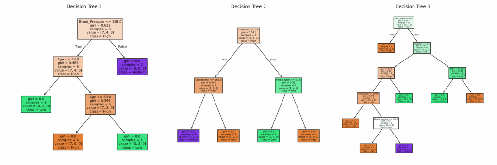
Using Random Forest to Make Predictions
Now we’ll use the model to make predictions on the test dataset. We’ll display the actual and predicted Disease Risk values for several cases.
# ==============================
# Step 5: Make Predictions on the Test Set
# ==============================
# Use the trained Random Forest model to predict the Disease Risk on the test set.
y_pred = rf.predict(X_test)

# Create a DataFrame to compare actual and predicted values.
results_df = X_test.copy()
results_df["Actual_Disease_Risk"] = y_test
results_df["Predicted_Disease_Risk"] = y_pred

# Display the first few rows of the results.
print("=== Predictions vs. Actual (Test Set) ===")
print(results_df.head())
print("\n")Evaluating Random Forest Performance
Finally, we evaluate the model’s performance.
# ==============================
# Step 6: Evaluate the Model Performance
# ==============================
# Calculate the overall accuracy of the model.
accuracy = accuracy_score(y_test, y_pred)
print(f"Model Accuracy: {accuracy:.2f}")

# Compute the confusion matrix to see the counts of true positives, false positives, etc.
conf_matrix = confusion_matrix(y_test, y_pred, labels=rf.classes_)

# Create a heatmap of the confusion matrix using seaborn for better visualization.
plt.figure(figsize=(6, 5))
sns.heatmap(conf_matrix, annot=True, fmt="d", cmap="Blues",
            xticklabels=rf.classes_, yticklabels=rf.classes_)
plt.xlabel("Predicted Disease Risk")
plt.ylabel("Actual Disease Risk")
plt.title("Confusion Matrix")
plt.show()

# Generate a detailed classification report that includes precision, recall, and F1-score for each class.
class_report = classification_report(y_test, y_pred)
print("=== Classification Report ===")
print(class_report)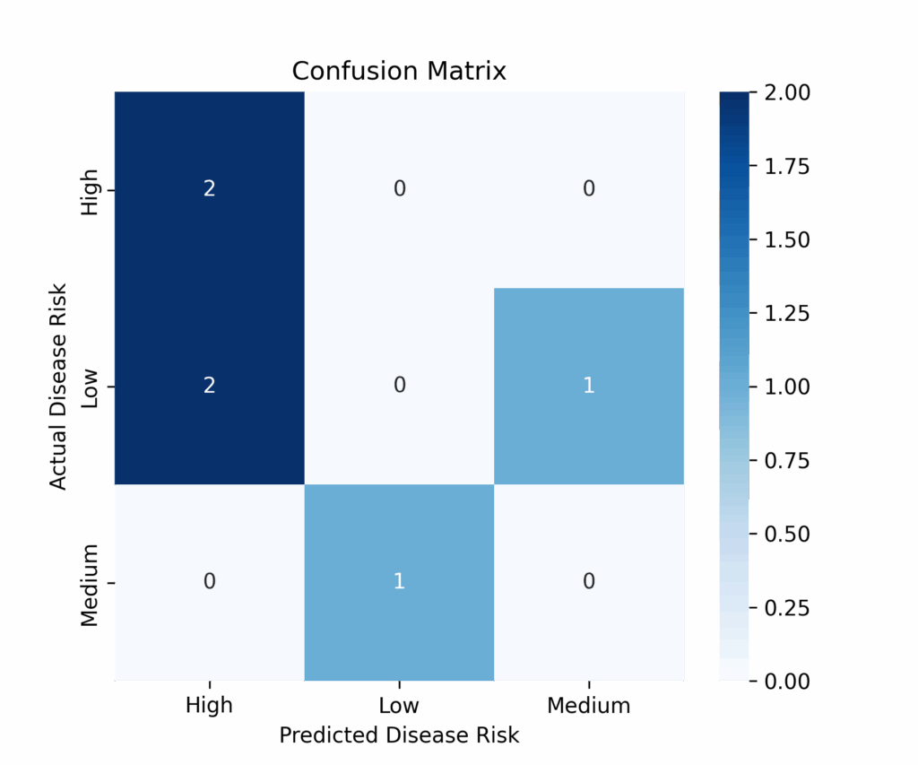
The model accuracy is very low (0.33). This is expected because, for educational purposes, we used a small dataset with few cases and created a forest with only three trees. This scenario isn’t ideal for Random Forest, which typically performs better with larger datasets (over 1000 cases) and forests containing hundreds or thousands of trees. Additionally, since we generated the dataset completely randomly, there are no meaningful patterns for the algorithm to learn from the features.
Feature importance in Random Forest
An important step in applying the Random Forest algorithm is evaluating the impact of different features on the model’s decisions. This evaluation helps us:
- understand which features have the greatest impact on the final decision
- eliminate less important features to streamline the model
- assess the impact of feature reduction on model performance
Feature importance can be calculated in different ways:
- Gini importance (based on the reduction of impurity at tree nodes: the more a feature reduces impurity, the more important it is)
- Permutation importance (randomly swaps feature values and evaluates changes in model performance)
Feature importance evaluation occurs after training the model with all available features. Once calculated, less relevant features may be removed, followed by new model training to compare performance.
Let’s create a fake medical dataset and perform feature importance evaluation using the two methods mentioned:
# Import necessary libraries
import numpy as np
import pandas as pd
import matplotlib.pyplot as plt
import seaborn as sns
from sklearn.ensemble import RandomForestClassifier
from sklearn.model_selection import train_test_split
from sklearn.metrics import accuracy_score
from sklearn.inspection import permutation_importance

# Step 1: Create a Synthetic Medical Dataset
np.random.seed(42)

# Generate synthetic patient data
num_samples = 500  # Number of patients

# Features: Age, Blood Pressure, Cholesterol Level, Heart Rate, Diabetes (1=Yes, 0=No)
age = np.random.randint(30, 80, num_samples)
blood_pressure = np.random.randint(100, 180, num_samples)
cholesterol = np.random.randint(150, 300, num_samples)
heart_rate = np.random.randint(60, 100, num_samples)
diabetes = np.random.choice([0, 1], size=num_samples, p=[0.7, 0.3])  # 30% have diabetes

# Target Variable: Heart Disease (1=Yes, 0=No) - Based on thresholds
heart_disease = (cholesterol > 250) | (blood_pressure > 160) | (diabetes == 1)
heart_disease = heart_disease.astype(int)

# Create a DataFrame
medical_data = pd.DataFrame({
    'Age': age,
    'BloodPressure': blood_pressure,
    'Cholesterol': cholesterol,
    'HeartRate': heart_rate,
    'Diabetes': diabetes,
    'HeartDisease': heart_disease
})

# Step 2: Split the Data into Training and Testing Sets
X = medical_data.drop(columns=['HeartDisease'])  # Features
y = medical_data['HeartDisease']  # Target variable

X_train, X_test, y_train, y_test = train_test_split(X, y, test_size=0.2, random_state=42, stratify=y)

# Step 3: Train the Random Forest Classifier
rf_model = RandomForestClassifier(n_estimators=200, max_depth=10, random_state=42)
rf_model.fit(X_train, y_train)

# Step 4: Evaluate the Model
y_pred = rf_model.predict(X_test)
accuracy = accuracy_score(y_test, y_pred)
print(f"Model Accuracy: {accuracy:.2f}")

# Step 5: Compute Feature Importance using Gini Importance
feature_importance_gini = pd.DataFrame({
    'Feature': X_train.columns,
    'Importance': rf_model.feature_importances_
}).sort_values(by='Importance', ascending=False)

# Step 6: Compute Feature Importance using Permutation Importance
perm_importance = permutation_importance(rf_model, X_test, y_test, n_repeats=10, random_state=42)

feature_importance_perm = pd.DataFrame({
    'Feature': X_train.columns,
    'Importance': perm_importance.importances_mean
}).sort_values(by='Importance', ascending=False)

# Step 7: Visualize Feature Importance (Gini Importance)
plt.figure(figsize=(8, 5))
sns.barplot(x=feature_importance_gini['Importance'], y=feature_importance_gini['Feature'])
plt.title("Feature Importance - Random Forest (Gini Importance)")
plt.xlabel("Importance Score")
plt.ylabel("Feature")
plt.show()

# Step 8: Visualize Feature Importance (Permutation Importance)
plt.figure(figsize=(8, 5))
sns.barplot(x=feature_importance_perm['Importance'], y=feature_importance_perm['Feature'])
plt.title("Feature Importance - Random Forest (Permutation Importance)")
plt.xlabel("Importance Score")
plt.ylabel("Feature")
plt.show()

# Display Feature Importance DataFrames
print("\nFeature Importance (Gini Importance):")
print(feature_importance_gini)

print("\nFeature Importance (Permutation Importance):")
print(feature_importance_perm)
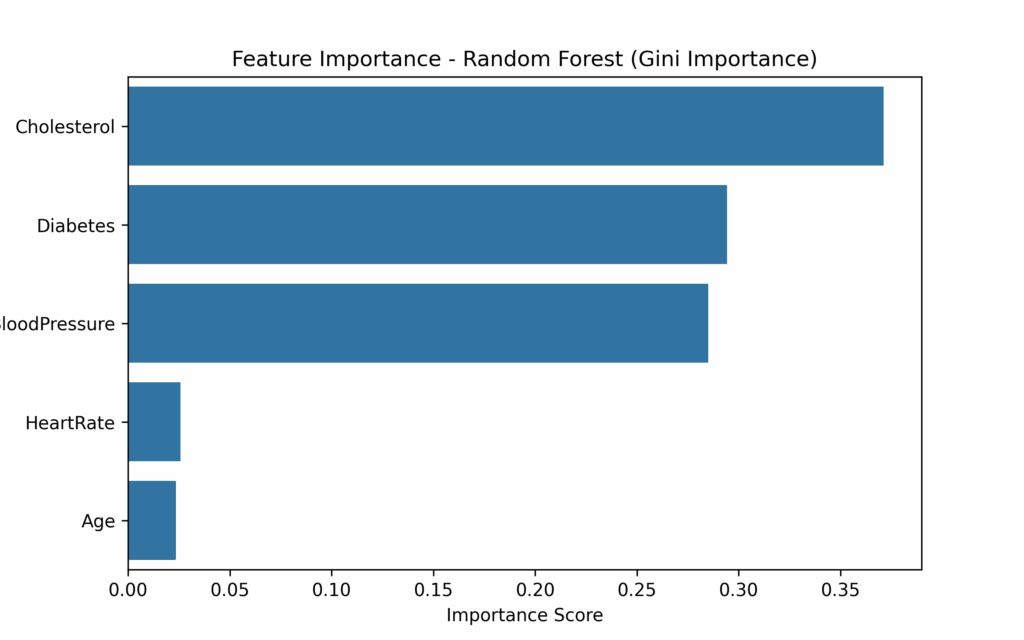
As shown in the feature importance graph, HeartRate and Age contribute minimally to the final prediction. The logical next step would be to remove these two features and retrain the model to assess whether its performance improves.
Where can you learn more about Random Forest?
What Is Random Forest? | IBMhttps://careerfoundry.com/en/blog/data-analytics/what-is-random-forest
Random Forest Algorithmhttps://builtin.com/data-science/random-forest-algorithm
Random Forests in ML for Advanced Decision-Making
Conclusion
The Random Forest algorithm is an ensemble learning method based on bagging, known for its high accuracy, robustness, and resistance to overfitting compared to individual decision trees. Compared to algorithms like SVM, k-NN, and neural networks, it offers a good compromise between performance and interpretability, proving particularly effective with structured data containing many features. However, it is less interpretable than a single decision tree and less efficient than linear models when the dataset is very large. Algorithms like Gradient Boosting (XGBoost, LightGBM) often outperform Random Forest in accuracy on complex problems, though they require more optimization.