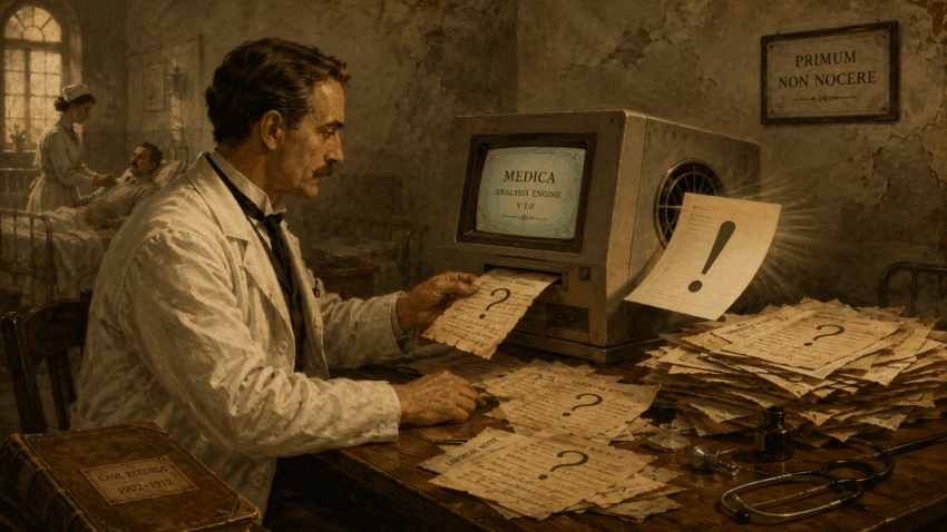
Doctor in a vintage hospital ward feeds a medical report marked with a question mark into an old computer, which returns the same sheet with a green exclamation mark.

How Well Can a Local 30B Model Answer Medical Questions? Benchmarking Meta Muse Glimmer on an RTX 3090

Posted on August 20, 2026August 20, 2026 by Michele Danilo Pierri

A reproducible 300-question evaluation across medical exams, biomedical literature, multilingual question answering, and clinical calculation

Meta released Muse Glimmer on 10 August 2026: thirty billion parameters, open weights, built for agentic work on consumer hardware.[1,2] I tested a quantized version five days later on a single NVIDIA RTX 3090 — partly because it was the first release in months whose size and quantization looked like a comfortable fit for 24 GB of VRAM rather than a fight with it, partly because I had a few free hours.

Whether a language model can replace clinical judgment is not something a benchmark settles, and I did not set out to ask it. My question was narrower: how accurately and reliably can this new general-purpose model answer a diverse set of established medical benchmark questions when it runs entirely on a personal workstation? That much a benchmark can address, at least in part.

Encouraging, and uneven. Muse Glimmer answered 248 of 300 questions correctly, for a pooled accuracy of 82.7% (Wilson 95% confidence interval, 78.0%–86.5%). Its macro-average across six benchmark families was 82.8%. Every response came back in the required structured format :no invalid outputs, no truncated generations, no parsing failures.

The headline number hides a clinically important pattern, though, and I should also say at the outset that I distrust benchmark scores this high. Both points I come back to below. Performance reached 98% on the MedQA sample and 92.5% on MedExpQA, including 90% on the Italian subset. It fell to 74% on clinical calculation and PubMedQA, and to 70% on MedMCQA. Inside MedCalc-Bench, formula-based physical and laboratory calculations were usually correct; rule-based risk scores were much less reliable. That contrast matters more than the overall ranking.

Key result: Muse Glimmer 30B Q4KM achieved 82.7% accuracy on 300 medical benchmark questions when run locally on an RTX 3090, with 0 invalid responses and a median end-to-end latency of 6.94 seconds per question.

Why test a local general-purpose model on medicine?

Medical language-model evaluations have traditionally focused on very large proprietary systems, or on models specifically adapted to medicine. MultiMedQA helped establish the modern pattern of combining examination questions, biomedical research questions, and consumer health tasks in a single broader framework.[3] Newer benchmarks have pushed into multilingual assessment, clinical calculations, electronic health records, and real-world workflows.

Local models raise a different practical question, and it is the one I have been working on for some time. A model that runs on one workstation can be evaluated without sending a single prompt to a cloud service. Infrastructure costs are predictable. It works without network access, and it can be dropped into experimental workflows where local control matters. None of that establishes clinical safety — it does make independent, reproducible testing considerably easier.

What makes Muse Glimmer interesting is precisely that Meta did not release it as a medical model. It is a dense 30-billion-parameter causal language model, distilled from a larger teacher, optimized for agentic tasks, tool use, multimodal understanding, and long-running local workflows.[1,2] Testing it on medicine therefore asks whether general reasoning capability transfers into a demanding domain that was never the stated target.

Methods

Model and local hardware

The evaluated model was Meta Muse Glimmer 30B in GGUF Q4KM quantization. Inference ran locally on Windows 11, on an NVIDIA RTX 3090 with 24 GB of VRAM and 64 GB of system RAM. The model was served through the OpenAI-compatible endpoint of llama-server, using the NVIDIA CUDA build of llama.cpp version 0.1.0-dev, build 10437, commit 16d222fc5.[4]

Runtime context length was 8,192 tokens. All model layers were offloaded to the GPU. Observed model allocation was approximately 18.0 GB of VRAM, which left enough headroom for the context and runtime buffers.

I heard the thermal problem before I measured it. During an initial pilot at the card’s 350 W default limit the fans went to 100% and stayed there; when I finally looked, the core had settled at 88–89 °C. I stopped the run, discarded those responses, and restarted from zero with a fixed 280 W power limit, 80% of the default board limit. Under sustained inference the core then stabilized around 80–82 °C, with fan speed near 68% in the monitored block. The final 300-question dataset therefore contains only responses generated under the 280 W configuration.

Benchmark composition

The test set was a reproducible stratified sample of 300 questions generated with sampling seed 20260813, combining six established benchmark families:

Benchmark	Questions	Domain
MedQA	50	US medical licensing-style multiple-choice questions
MedMCQA	50	Multi-subject Indian medical entrance-examination questions
PubMedQA	50	Yes/no/maybe inference from biomedical research abstracts
MedCalc-Bench Verified	50	Rule-based and equation-based clinical calculations
MedExpQA	40	Medical exam questions with gold explanations: 20 English and 20 Italian
MMLU medical subsets	60	Ten questions from each of six medical and biological subjects
Total	300

MedQA was introduced as a multilingual open-domain medical examination dataset.[5] MedMCQA contains more than 194,000 questions drawn from AIIMS and NEET-PG examinations across 21 medical subjects.[6] PubMedQA tests whether a model can infer a yes, no, or maybe answer from biomedical research text.[7] The MMLU subsets covered anatomy, clinical knowledge, college biology, college medicine, medical genetics, and professional medicine.[8]

Two features drew me to MedExpQA, both of them scarce in medical benchmarks: multilingual questions, and gold explanations written by physicians.[9] MedCalc-Bench asks for something different again — extracting clinical variables, then applying equations or rule-based scores.[10] I used the maintained MedCalc-Bench Verified dataset rather than the deprecated earlier versions, for reasons that turn out to matter (see below).[11]

Inference protocol

Inference was zero-shot and sequential. During generation the runner had access only to the question file; the answer key and scoring records stayed separate until inference had finished. Principal generation settings:

Parameter	Value
Temperature	0
Top-p	1
Seed	42
Maximum completion tokens	2,048
Reasoning strength	Low
Context length	8,192
Timeout	180 seconds
Retries	2
Concurrent requests	1

A machine-readable final answer was required by the output contract. Multiple-choice datasets returned the selected option, PubMedQA returned yes, no, or maybe, and MedCalc-Bench returned a numerical or date result. Responses were written to JSONL immediately, so that an interrupted run could resume without repeating successful questions.

For thermal control and operational recovery the evaluation ran in six blocks of 50 questions, with the card allowed to fall below 50 °C between blocks before the next one started. Overcautious, probably. It cost a few minutes per block and removed a variable I did not want to be arguing about afterwards. Model, prompt, generation parameters, power limit, and output file were identical across blocks.

Scoring and statistical analysis

MedQA, MedMCQA, PubMedQA, MedExpQA, and MMLU were scored by normalized exact match. MedCalc-Bench decimal and integer outputs counted as correct when the parsed numerical value fell within the inclusive lower and upper limits supplied by the verified source dataset; date outputs used the corresponding inclusive date interval.

Primary descriptive outcomes were pooled accuracy and macro-average accuracy across benchmark families, with Wilson 95% confidence intervals for proportions. The macro-average weights each of the six families equally; pooled accuracy weights every question equally. Operational outcomes were invalid-response rate, end-to-end latency, and completion-token throughput.

Results

Overall performance

Muse Glimmer answered 248 of 300 questions correctly. Pooled accuracy was 82.7%, the equal-weighted macro-average 82.8%. That the two values sit almost on top of each other indicates the overall result was not materially driven by the slightly different sample sizes between datasets.

All 300 generations carried status: ok, finish_reason: stop, and a valid parsed answer. No duplicated question identifiers. Invalid-response rate: 0%.

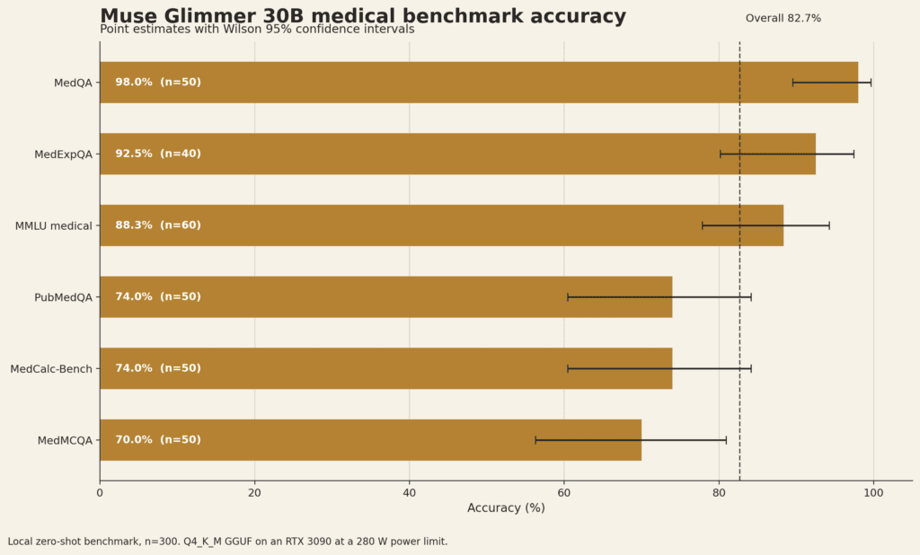
Accuracy of Muse Glimmer 30B across six medical benchmarks, with Wilson 95% confidence intervals.

Accuracy differed substantially by benchmark

Dataset	Correct / N	Accuracy	Wilson 95% CI
MedQA	49/50	98.0%	89.5%–99.6%
MedExpQA	37/40	92.5%	80.1%–97.4%
MMLU medical	53/60	88.3%	77.8%–94.2%
MedCalc-Bench	37/50	74.0%	60.4%–84.1%
PubMedQA	37/50	74.0%	60.4%–84.1%
MedMCQA	35/50	70.0%	56.2%–80.9%

MedQA produced the strongest result by a distance: one miss in fifty. MedExpQA and the medical MMLU subsets also gave high point estimates. MedMCQA was weakest, with 15 errors, while MedCalc-Bench and PubMedQA contributed 13 each.

Between them, MedMCQA, MedCalc-Bench, and PubMedQA accounted for 41 of the 52 total errors (78.8%). Such a concentration suggests that an overall medical QA score is not enough to characterize model behaviour. Examination-style recall, literature inference, and clinical computation stress genuinely different capabilities.

English and Italian MedExpQA

Nineteen of 20 English MedExpQA questions were answered correctly (95%), and 18 of 20 Italian ones (90%). Five points of difference across 20 questions per language is not a finding; the confidence intervals are wide and strongly overlapping, and I would not build anything on it.

The Italian result is still useful in a weaker sense. It shows the model’s strong MedExpQA performance was not confined to English in this sample. A proper multilingual evaluation would need the complete MedExpQA test set and prespecified paired language comparisons.

MedExpQA language	Correct / N	Accuracy
English	19/20	95.0%
Italian	18/20	90.0%

MMLU medical subjects

Across the six MMLU subsets, performance ranged from 70% to 100%:

MMLU subject	Correct / N	Accuracy
College biology	10/10	100%
Medical genetics	10/10	100%
Clinical knowledge	9/10	90%
Professional medicine	9/10	90%
College medicine	8/10	80%
Anatomy	7/10	70%

Descriptive only, these. With ten questions per subject a single answer moves the estimate ten percentage points, so the ordering should not be read as a ranking. The distribution is nevertheless helpful for choosing which domains deserve larger confirmatory samples: anatomy and college medicine are the natural targets for error analysis.

Clinical calculation exposed a specific weakness

Aggregate MedCalc-Bench accuracy was 74%. The category-level breakdown is sharply heterogeneous:

MedCalc category and output	Correct / N	Accuracy
Physical, decimal	13/13	100%
Laboratory test, decimal	16/17	94.1%
Dosage, integer	2/3	66.7%
Severity, integer	2/3	66.7%
Risk, integer	4/12	33.3%
Risk, decimal	0/2	0%

Subgroup sizes here are small, particularly for dosage, severity, and decimal risk. The error pattern is clinically plausible all the same, and worth pursuing. Continuous formula-based calculations went well; rule-based risk scores, which require correctly extracting several criteria, assigning points, and summing them, did not. One case was a CHA₂DS₂-VASc calculation where the model returned 3 against a verified score of 5.

Worth pausing on that one. Both values sit above the usual anticoagulation threshold, so in that particular case the downstream decision would probably not have changed — which is exactly the kind of near-miss that makes an aggregate accuracy figure feel reassuring and tell you nothing. I have not yet gone back through the raw outputs to identify which criteria the model dropped, and until someone does, “74% on clinical calculation” is a number without a mechanism behind it.

The wider point is that numerical ability should not be treated as one construct. Applying a direct equation to explicit measurements is a different task from identifying several clinical attributes buried in prose and mapping each to a scoring rule. A larger analysis would want to classify MedCalc errors into entity extraction, rule selection, arithmetic, unit conversion, and final-answer formatting.

Latency and throughput

Median end-to-end latency was 6.94 seconds per question, with a 90th percentile of 16.77 seconds. Median completion throughput, calculated end to end, was 29.96 tokens per second.

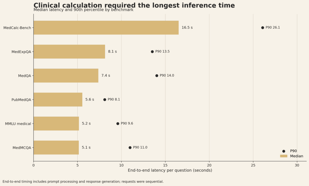
MedCalc-Bench demanded the longest responses and the most inference time — median latency 16.51 seconds, against roughly five to eight seconds elsewhere.

Dataset	Median latency	P90 latency
MedMCQA	5.14 s	10.98 s
MMLU medical	5.16 s	9.55 s
PubMedQA	5.55 s	8.05 s
MedQA	7.38 s	13.98 s
MedExpQA	8.13 s	13.51 s
MedCalc-Bench	16.51 s	26.06 s

Median and 90th-percentile end-to-end latency for Muse Glimmer 30B across six medical benchmarks.

Capping the board power reduced thermal stress while preserving practical throughput — a trade I would make again. None of these latency figures should be assumed to generalize to other quantizations, context sizes, GPU models, drivers, or inference-engine versions.

What the 82.7% score does (and does not) mean

Read correctly, the result says this: Muse Glimmer achieved 82.7% accuracy on a specific stratified sample of public medical benchmarks, under a documented local inference configuration.

It does not say the model has 82.7% diagnostic accuracy, that it is safe for clinical use, or that it can replace a clinician. Multiple-choice examinations and constrained final-answer tasks capture a thin slice of the clinical process. They do not test longitudinal synthesis, uncertainty communication, patient preferences, physical examination, workflow integration, or what happens when a recommendation is wrong.

Which brings me to the 98% on MedQA, and to a wider unease. I am always suspicious when a result is this good. I have argued elsewhere that a good deal of medical AI evaluation is quietly circular: the corpora used to train these systems and the corpora used to test them overlap, nobody outside the developing lab can say by how much, and the leaderboard rewards precisely that overlap. The other half of the pattern is just as visible — systems that look excellent on public benchmarks routinely perform considerably worse once they meet real clinical data. [Link to your earlier article on medical AI evaluation goes here.]

MedQA fits the description almost too neatly. Public, heavily reused, old enough to have been absorbed several times over. Meta does not disclose the complete training dataset, so contamination cannot be excluded here either. Genuine transfer, familiarity with the format, outright memorization: the 98% is compatible with all three, and from outside there is no way to separate them. Recent benchmark audits make a similar argument in more measured language, adding label quality and weak governance to the list of things that inflate medical leaderboard results.[12]

The same caution applies to comparing this run against published model scores. Prompt format, answer extraction, dataset version, quantization, inference framework, tool access — each of them moves performance. MedCalc-Bench is especially sensitive to version and scoring choices, since deprecated releases contained corrected labels and implementations. Hence the Verified dataset.[10,11]

Strengths

This pilot has several methodological strengths:

The answer key was isolated during inference. The runner read only the question file, and predictions were joined to gold answers afterwards.
The sample was reproducible. Dataset allocation and sampling seed were fixed in advance.
Inference was local and sequential. No cloud model, no web search, no retrieval system, no external clinical calculator.
Every raw output was preserved. Question-level auditing remains possible, rather than reliance on an aggregate score.
Scoring was deterministic. Normalized exact match for multiple-choice tasks; source-provided limits for MedCalc.
Operational reliability was measured, not assumed. All 300 responses terminated normally and parsed successfully.
The deployment configuration was recorded in full. Model quantization, GPU, runtime, context, power limit, decoding settings.

Limitations

The evaluation also has important limitations, and some of them are severe.

Three hundred questions are enough for a technical pilot and nowhere near enough for definitive model ranking. Dataset-specific confidence intervals stay wide, and the language and subject subgroups are far smaller still. My complete local benchmark contains 8,895 records and would support substantially more precise estimates; I simply did not have the GPU hours.

Then there is the fact that one model, one quantization, one hardware configuration, and one inference engine were tested. The result belongs to the whole deployment configuration, not to some abstract base model. Q4KM quantization may itself alter accuracy relative to higher-precision weights, and by how much I cannot say from a single run.

The prompt included Muse Glimmer’s low reasoning-strength instruction. Appropriate for a single-model pilot; not a neutral prompt for cross-model comparison. Any comparative study needs a model-agnostic primary prompt frozen before a second model is evaluated, with model-specific recommended prompts reserved for a secondary “best configuration” analysis.

Deterministic decoding was used once per question, and only once. Repeatability should be confirmed on a prespecified subset even at temperature zero — I would not assume it.

More fundamentally, this study scored final answers rather than the clinical validity of reasoning. A correct answer can sit on top of flawed reasoning, and an incorrect benchmark answer occasionally reflects an ambiguous or plainly wrong gold label. Separating knowledge deficits, extraction failures, arithmetic mistakes, questionable labels, and clinically unsafe reasoning would require blinded physician review.

And public benchmark performance says nothing at all about calibration, abstention, hallucination in open-ended responses, demographic bias, guideline currency, or real-world patient safety.

From rapid benchmark to research programme

This started as a rapid evaluation of a newly released model, run in the gaps of a working week. The result supports something more rigorous: a paired study of open-weight models that fit on a single 24 GB consumer GPU.

A confirmatory protocol should be frozen before the next model is touched. It needs to specify model inclusion criteria, exact dataset versions, a neutral prompt, quantization, context length, power limit, inference-engine build, primary and secondary outcomes, multiplicity correction, and the handling of invalid responses. All models answer the same questions, which permits paired comparison with McNemar tests and stratified bootstrap confidence intervals for accuracy differences.

Blinded clinical error review would be the strongest extension. Two clinicians, independently classifying a stratified sample of discordant or incorrect responses into knowledge, interpretation, entity extraction, rule selection, arithmetic, unit, and benchmark-label errors. That moves the work off the leaderboard and towards an account of where locally deployable models fail.

Conclusion

Muse Glimmer 30B delivered strong medical benchmark performance on a single consumer GPU: 248 of 300 questions correct, no invalid outputs, median latency below seven seconds at a 280 W power limit. Its best results came from MedQA, MedExpQA, and the medical MMLU subsets. Its worst came from MedMCQA, and from tasks requiring biomedical inference or rule-based clinical risk calculation.

The 82.7% is the least interesting number in this article. What the run actually showed is that a single aggregate score conceals a jagged capability profile — highly capable on familiar medical examination formats, considerably less reliable once clinical information had to be converted into a multivariable risk score. Which is the argument for multidomain, versioned, question-level evaluation, and for treating any headline medical benchmark figure, this one included, with more suspicion than it usually receives.

Frequently asked questions

Can Muse Glimmer 30B run on an RTX 3090?

Yes. The Q4KM GGUF used here occupied approximately 18 GB of the RTX 3090’s 24 GB VRAM at an 8,192-token context. Exact requirements depend on quantization, context, runtime buffers, and any optional multimodal components.

What medical benchmark score did Muse Glimmer achieve?

82.7% pooled accuracy and 82.8% macro-average accuracy on this stratified 300-question sample. The 95% Wilson confidence interval for pooled accuracy was 78.0%–86.5%.

Was the model connected to the internet or external tools?

No. Inference was local, sequential, and closed-book — no web search, no retrieval-augmented generation, no clinical calculator.

Does this result show that Muse Glimmer is clinically safe?

No. It measures performance on public benchmark questions. Not diagnostic safety, not treatment quality, not calibration, and not performance in patient care.

Why was the GPU power limited to 280 W?

The stock 350 W pilot produced sustained core temperatures of 88–89 °C at maximum fan speed, so I discarded it. Restarting at 280 W brought the sustained core temperature down to roughly 80–82 °C while retaining practical inference speed. The definitive run was also split into six blocks of 50 questions, with the card cooling below 50 °C between blocks.

References

Meta AI. Introducing Muse Glimmer: An Open Agentic Model That Runs on a Single GPU. Published 10 August 2026.
Meta. Muse Glimmer 30B model card. Hugging Face; 2026.
Singhal K, Azizi S, Tu T, et al. Large language models encode clinical knowledge. Nature. 2023;620:172–180. doi:10.1038/s41586-023-06291-2.
Gerganov G, llama.cpp contributors. llama.cpp: LLM inference in C/C++. GitHub.
Jin D, Pan E, Oufattole N, Weng WH, Fang H, Szolovits P. What Disease Does This Patient Have? A Large-Scale Open Domain Question Answering Dataset from Medical Exams. Applied Sciences. 2021;11(14):6421. doi:10.3390/app11146421.
Pal A, Umapathi LK, Sankarasubbu M. MedMCQA: A Large-scale Multi-Subject Multi-Choice Dataset for Medical Domain Question Answering. Proceedings of the Conference on Health, Inference, and Learning. 2022;174:248–260.
Jin Q, Dhingra B, Liu Z, Cohen WW, Lu X. PubMedQA: A Dataset for Biomedical Research Question Answering. Proceedings of EMNLP-IJCNLP. 2019:2567–2577. doi:10.18653/v1/D19-1259.
Hendrycks D, Burns C, Basart S, et al. Measuring Massive Multitask Language Understanding. International Conference on Learning Representations. 2021.
Alonso I, Oronoz M, Agerri R. MedExpQA: Multilingual Benchmarking of Large Language Models for Medical Question Answering. Artificial Intelligence in Medicine. 2024;155:102938. doi:10.1016/j.artmed.2024.102938.
Khandekar N, Jin Q, Xiong G, et al. MedCalc-Bench: Evaluating Large Language Models for Medical Calculations. Advances in Neural Information Processing Systems. 2024;37.
Khandekar N, et al. MedCalc-Bench Verified. Maintained dataset repository; accessed August 2026.
Chen W, Yu G, Cheung YF, et al. Beyond the Leaderboard: Rethinking Medical Benchmarks for Large Language Models. Accepted at ACL 2026; arXiv:2508.04325.

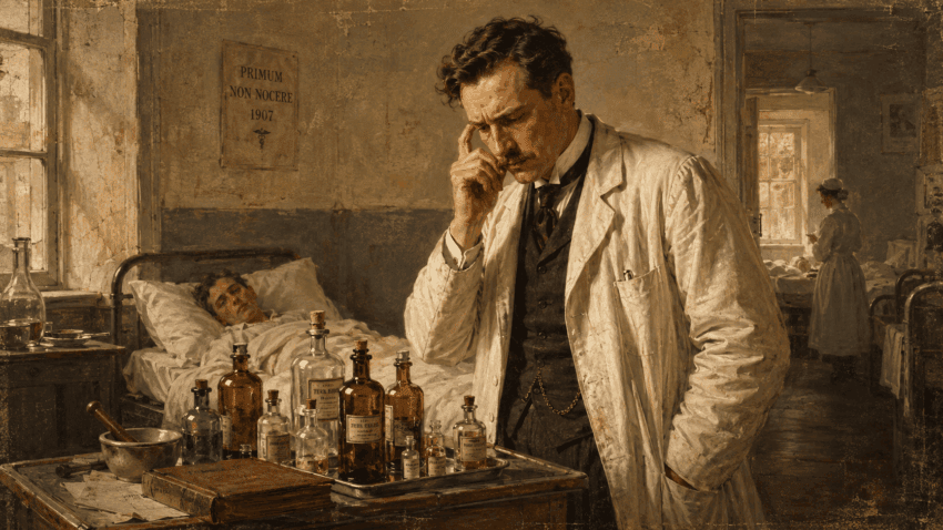
Early 20th-century doctor looks perplexed at a bedside table crowded with medicine vials and bottles in an old hospital ward.

From Chart to Variable: Extracting Computable Clinical Features from the EHR

Posted on August 16, 2026August 16, 2026 by Michele Danilo Pierri

Vasoactive-Inotropic Score as a Worked Example

Introduction: The Data Is There. The Variable Is Not.

Every conversation about clinical AI opens on the same premise: hospitals are sitting on enormous quantities of data. True enough, and almost useless as a starting point. An electronic health record is a transactional system, built for documentation, for billing, and for medico-legal defence — three purposes, none of them research. It was never designed to emit variables. It emits events, and an event is not a measurement.

Take the hardest table in a cardiac surgical ICU, which is the infusion record. Open it for one patient on postoperative day zero. Four or five drugs running concurrently. Norepinephrine in micrograms per kilogram per minute; vasopressin in units per minute, or units per kilogram per minute, depending on who configured the pump library and when. Milrinone at a rate nobody has touched since the patient left theatre. Two rows for the same drug at 03:14, because a pump was swapped. A retrospective correction entered at 07:00 by the night nurse. And somewhere in there, a dose documented in mL/h whose concentration lives in a free-text order comment.

Everything a researcher would want to know about hemodynamic support is in that table. Almost none of it is in a form that a regression, a Cox model or a transformer can consume.

The distance between “we have the data” and “we have a dataset” is where clinical informatics does most of its actual work, and the standard instrument for closing it is the derived clinical variable: a hand-specified function mapping a messy, irregularly sampled, multi-unit set of events onto a single interpretable number. The Vasoactive-Inotropic Score (VIS) and the norepinephrine equivalent dose (NEE) are two such functions. Same raw material, different assumptions, different answers.

I use them here as a case study. The clinical content matters, but what I am really arguing about is the transformation.

The Derived Clinical Variable as a Design Pattern

Anyone who has built an ICU dataset has reinvented this pattern without giving it a name. SOFA, APACHE II, SAPS, the Charlson index, the VIS — structurally the same object. A clinician-specified projection from a high-dimensional, ragged, partially observed event stream onto a low-dimensional vector that some downstream method can actually handle.

Three properties of raw infusion data make it resistant to direct modelling. The derived variable takes them one at a time.

Unit heterogeneity. Six drugs, four unit systems, and at least two documentation conventions for the same agent. No arithmetic is possible until this is resolved — and resolving it is not a data-cleaning step. It is a clinical decision about what counts as an equivalent dose.
Irregular, informative sampling. Rates get recorded when someone changes them, or when a nurse charts a shift observation. Never on a fixed grid. The sampling pattern itself carries information about how sick the patient is, which turns out to be a problem in its own right; I come back to it below.
Dimensionality with treatment-driven correlation. Six drug channels, mostly zero, heavily correlated because they reflect a single escalation policy rather than six independent decisions. Hand a model the raw channels and it will spend much of its capacity relearning that policy.

The alternative to hand-crafting is to feed the raw multivariate series into a sequence model and let it build its own representation. On large datasets that works, and sometimes works better. What it costs is interpretability, portability across institutions, and the ability to state in a methods section what was actually measured. For most clinical research — and for anything that will eventually face a regulator or a reviewer — the hand-crafted feature is still the pragmatic option. My only insistence is that it be treated as a choice, with consequences, argued for rather than inherited from whatever the last paper in the field happened to do.

Case Study One: The VIS as a Compression Function

The VIS descends from the inotrope score of Wernovsky and colleagues, defined in 1995 inside a randomized comparison of low-flow bypass against circulatory arrest for the arterial switch operation [4]:

Inotrope score = dopamine (µg/kg/min) + dobutamine (µg/kg/min) + 100 × epinephrine (µg/kg/min)

Gaies and colleagues extended it in 2010 to the drugs a modern pediatric cardiac ICU actually uses, and validated the result against outcome [5]:

VIS =
Dopamine (µg/kg/min)

Dobutamine (µg/kg/min)

100 × Epinephrine (µg/kg/min)

100 × Norepinephrine (µg/kg/min)

10 × Milrinone (µg/kg/min)

10 000 × Vasopressin (units/kg/min)

Read structurally rather than clinically, that is a fixed linear projection from a six-dimensional dose vector onto a scalar, with weights chosen once and never fitted. It is the framing I would keep in mind throughout, because it makes the design assumptions visible.

Worked example, infant on postoperative day zero:

Agent	Dose	Weight	Contribution
Norepinephrine	0.08 µg/kg/min	×100	8
Epinephrine	0.05 µg/kg/min	×100	5
Milrinone	0.5 µg/kg/min	×10	5
Vasopressin	0.0005 U/kg/min	×10 000	5
		VIS	23

The weights are conventions. They are not pharmacology. Of everything written about this score, that is the point most consistently misreported. The multipliers were assigned so the arithmetic would stay easy, and so that agents used at wildly different absolute doses would land in a comparable numerical range. Belletti and colleagues say so without hedging: the correction factors were attributed arbitrarily to permit simple calculation and may not reflect real equipotency [6].

For anyone building a model, this is a specification rather than a defect. It makes the VIS a stable, reproducible convention rather than a physiological measurement, and it should be documented in a methods section the way one documents a normalisation constant — not the way one documents a lab assay. A VIS of 20 driven entirely by norepinephrine and a VIS of 20 driven by milrinone plus low-dose dopamine are the same number describing two rather different patients. Lossy compression, then, but lossy in a specific and knowable direction.

Case Study Two: The NEE, or the Same Problem Solved Differently

General critical care converged on a different function over the same raw data. The norepinephrine equivalent dose asks a narrower question — how much vasopressor is this patient on, expressed in norepinephrine-equivalent terms — and answers it with ratios taken from comparative potency studies rather than assigned by fiat. Goradia and colleagues synthesised 21 such studies into a working formula [7]; Kotani and colleagues later extended it into an updated NEE score covering the agents that have entered practice since [8].

Two functions, one dataset, different design commitments:

	VIS	NEE
Scope	Vasopressors and inotropes	Vasopressors only
Weights	Assigned by convention (2010)	Partly derived from potency studies
Measures	Total cardiovascular pharmacological support	Vasoconstrictor burden
Best fit	Postcardiotomy physiology, where inotropy and vasoconstriction coexist	Vasoplegic and septic shock; increasingly the standard for trial eligibility

What I find instructive is that neither is the true value of anything. They are two competing operationalisations of one latent construct — how much hemodynamic support is this patient receiving — and they will rank the same cohort differently. Once the infusion data are normalised, computing both costs almost nothing, and reporting both turns an arbitrary choice into a sensitivity analysis. I have come to treat that as the default for any study using either, though the literature has not caught up.

The Extraction Pipeline: Five Layers That Each Fail Differently

This is the part that gets compressed into a single sentence in most methods sections — “vasoactive doses were extracted from the EHR and the VIS was calculated” — and that determines, far more than any modelling choice downstream, whether the result means anything at all.

Layer 0. Source semantics: what does a row actually mean?

Before a line of code is written, someone has to establish what the source table records. Ordered? Administered? Documented? A medication administration record row can represent a prescription that was never hung, a rate that was set on the pump, or a nurse’s retrospective observation of what the pump was doing. Three different variables. Most systems mix them, and the mixture is rarely documented anywhere you can find it.

The companion question is what an absent row means. There is no record of norepinephrine between 04:00 and 08:00. Was the infusion off, or running unchanged and therefore not re-charted? The answer is institution-specific and it cannot be recovered from the data alone. It has to be established with the people who do the charting, which in practice means sitting down with the nursing coordinator rather than reading a data dictionary. Get this wrong and you have made the most consequential error in the whole pipeline — one that passes every downstream quality check without a murmur.

Layer 1. Concept normalisation

Local drug codes have to be resolved to a controlled vocabulary before anything is comparable across systems or sites. The mature answer is the OMOP Common Data Model with the OHDSI standardised vocabularies: drugs to RxNorm concepts, measurements to LOINC, conditions to SNOMED CT [1]. The practical payoff is that identical extraction code runs at every site holding data in the model, which is what makes federated multicentre analysis possible at all.

For anyone learning this, MIMIC-IV is still the most useful sandbox — a fully open ICU EHR extract from Beth Israel Deaconess, with published derived-concept code you can read, criticise and fork [2]. Reading someone else’s vasopressor extraction against a dataset you can also download yourself is worth more than any amount of methodological reading. It certainly taught me more.

Layer 2. Dose harmonisation

Every VIS component wants µg/kg/min or U/kg/min. Source systems rarely oblige. This is the layer where clinical judgement travels in disguise, dressed as unit conversion.

Volumetric rates in mL/h need the drug concentration, sometimes structured, sometimes buried in an order comment. Then a weight — and there the question has no neutral answer. Admission weight, daily weight, or dry weight? In an edematous postoperative patient the three can differ by more than ten percent, and whichever you pick propagates into every score in the cohort. Pick one, state it, hold it constant.

Then the vasopressin trap, which deserves spelling out because it keeps recurring in published work. Pediatric cardiac practice doses vasopressin at roughly 0.0003 to 0.002 U/kg/min, so a typical infusion contributes 3 to 20 VIS points. Adults are prescribed a fixed rate in U/min, commonly 0.01 to 0.04, which has to be divided by body weight before the multiplier applies: for a 70 kg patient, 0.03 U/min works out to about 0.00043 U/kg/min, roughly 4 points. Feed an adult-convention value into a pediatric-convention formula and a plausible score of 23 becomes 300. In a cohort of ten thousand stays, nobody reads the outliers. The model does.

Any pipeline touching both populations has to handle the convention explicitly, per source system. Not inferred, and certainly not assumed.

Layer 3. Temporal reconstruction

Layers 0 to 2 leave you with a set of point events. What a model needs is a function of time. Three decisions bridge the two:

Interval reconstruction. Start times, stop times and rate changes become contiguous intervals of constant rate, per drug and per line.
Overlap resolution. Two concurrent entries for the same agent nearly always mean a pump swap or a double-documented change, not two genuine infusions. Sum them and you have silently doubled the dose. Deduplication rules belong in code, with the counts reported.
Projection onto a grid. Hourly maximum and hourly time-weighted mean are different operators, and they produce measurably different values of VIS_max. Neither is wrong. Choosing without declaring which is.

That last point travels well beyond this score. An aggregation operator is an inductive bias. A maximum encodes the belief that peak support is what matters; a time-weighted mean, that cumulative exposure matters; a slope, that trajectory matters. Clinical hypotheses, all three, wearing the costume of a data-processing step.

Layer 4. Feature derivation

Only now is the score computed, and it should be computed against a versioned coefficient table rather than a hard-coded expression. Coefficients drift — Belletti’s extended version, the various phenylephrine conventions, the NEE updates — and a study that cannot state which version it used cannot be replicated.

-- vis_coefficient(drug, coefficient, expected_unit, version)
-- infusion_normalised: output of layers 0-2, rates in ug/kg/min or U/kg/min

WITH gridded AS (
    SELECT
        patient_id,
        date_trunc('hour', charttime) AS hr,
        drug,
        MAX(rate_per_kg_min) AS rate        -- layer 3 decision: hourly maximum
    FROM infusion_normalised
    WHERE charttime >= :window_start
      AND charttime <  :window_end
    GROUP BY patient_id, date_trunc('hour', charttime), drug
)
SELECT
    g.patient_id,
    g.hr,
    SUM(g.rate * c.coefficient)                       AS vis,
    COUNT(*) FILTER (WHERE c.drug IS NULL)            AS unmapped_agents
FROM gridded g
LEFT JOIN vis_coefficient c
       ON c.drug    = g.drug
      AND c.version = 'gaies_2010'
GROUP BY g.patient_id, g.hr;

-- vis_coefficient(drug, coefficient, expected_unit, version)
-- infusion_normalised: output of layers 0-2, rates in ug/kg/min or U/kg/min

WITH gridded AS (
    SELECT
        patient_id,
        date_trunc('hour', charttime) AS hr,
        drug,
        MAX(rate_per_kg_min) AS rate        -- layer 3 decision: hourly maximum
    FROM infusion_normalised
    WHERE charttime >= :window_start
      AND charttime <  :window_end
    GROUP BY patient_id, date_trunc('hour', charttime), drug
)
SELECT
    g.patient_id,
    g.hr,
    SUM(g.rate * c.coefficient)                       AS vis,
    COUNT(*) FILTER (WHERE c.drug IS NULL)            AS unmapped_agents
FROM gridded g
LEFT JOIN vis_coefficient c
       ON c.drug    = g.drug
      AND c.version = 'gaies_2010'
GROUP BY g.patient_id, g.hr;

Two deliberate choices in that query. The join is a LEFT JOIN with an explicit count of unmapped agents, because a cohort in which fifteen percent of vasoactive exposure falls outside the coefficient table is a cohort where the VIS is quietly measuring something incomplete — and that number belongs in the paper, not in a code comment. Second, drugs outside the classic six are never folded in implicitly: where phenylephrine or levosimendan matter, generate parallel variables (vis_classic, vis_phe100, vis_phe10) so the coefficient choice surfaces as a reported sensitivity analysis rather than an assumption buried in a CASE statement.

The scalar is rarely the end point. Out of the same hourly series come the features that actually enter models: maximum over a window, time-weighted mean, slope or weaning rate, cumulative time above a threshold. VIS_max is the best validated of these and tells you least about trajectory.

Layer 5. Provenance

The extraction code is part of the method, not an implementation detail. Version the coefficient table, version the deduplication rules, record the grid resolution and the aggregation operator, publish the code alongside the paper. The alternative is what we have now, where two groups reporting “maximum VIS in the first 24 hours” may be computing quantities that differ by ten or twenty percent for reasons neither group can reconstruct.

What These Choices Do to Downstream Models

Here the extraction stops being plumbing and becomes epistemology. Four effects, each with a literature behind it.

1. Missingness is informative, and it leaks. Agniel, Kohane and Weber went through 272 laboratory tests across 669 452 patients and found something that ought to unsettle anyone building ICU models: for many tests, the timing of the order — hour of day, day of week, ordering frequency — predicted three-year survival better than the result did [3]. The healthcare process writes itself into the data. Applied here, the frequency with which an infusion rate gets re-charted is itself a marker of instability. Imputing “no record” as “no infusion” therefore does not merely lose information. It converts a strong predictor into a silent bias, which is worse.

2. The VIS is a treatment variable, and models learn treatment policy. The deepest issue on this list, and not specific to the VIS at all. The canonical illustration remains Caruana’s pneumonia model, which learned that asthma lowered mortality risk, because asthmatic patients were triaged straight to intensive care and treated aggressively [13]. The model had faithfully learned the treatment policy. Deployed, it would have killed people.

A VIS is a record of a decision. It measures what clinicians chose to prescribe in response to a patient they were watching, using information that is largely absent from the structured record. Include it as a predictor of mortality and the model is partly learning the local escalation protocol, partly learning the clinicians’ unrecorded gestalt. Sometimes that is exactly what you want — in a severity-adjustment model, for instance. It is precisely what you do not want in a causal analysis of a hemodynamic intervention, where the same variable is a time-varying confounder affected by prior treatment, and where standard adjustment will bias the estimate rather than repair it.

3. Prescribing culture becomes dataset shift. Two centres treating identical patients, one norepinephrine-first and one dopamine-first, will produce VIS distributions differing by an order of magnitude, with no difference whatever in physiology. Finlayson and colleagues catalogue precisely this class of failure: a model trained where the feature encodes local practice degrades wherever practice differs [14]. The external validation of the Epic Sepsis Model at Michigan Medicine — an AUC of 0.63 against a vendor-claimed 0.76 to 0.83, with substantial alert burden — remains the most widely cited demonstration that the concern is not theoretical [15].

The mitigation is unglamorous. Report the drug-mix distribution alongside the score, stratify or recalibrate by site, and treat any multicentre VIS-based model as requiring external validation before it means anything.

4. Convention beats optimality for portability. A weighting fitted on one cohort will outperform the 2010 coefficients on that cohort, and will not transfer. The arbitrary weights have one large compensating virtue: they are the same everywhere. For cross-study comparability, a stable convention is worth more than a locally optimal one — which is an argument, I think, for computing the classic VIS even when you also compute something better.

Does the Compression Retain Signal?

Having established that the VIS is lossy, convention-based and treatment-derived, the fair question is whether it survives contact with outcome data. It does. Moderate discrimination, which is about what a single hand-crafted scalar ought to buy.

Pediatric cardiac surgery. In the original Michigan cohort of 174 infants, a high maximum VIS over the first 48 postoperative hours carried an adjusted odds ratio of 8.1 (95% CI 3.4 to 19.2) for a composite poor outcome [5]. Multicentre confirmation across the PC4 and VPS registries, 391 infants, gave odds ratios of 6.5 (95% CI 2.9 to 14.6) for poor outcome and 13.2 (95% CI 3.7 to 47.6) for mortality [9]. Wide intervals, small cohorts — but the direction is not in doubt.
Adult cardiac surgery. Among 3213 patients, maximal VIS over 24 hours predicted a composite outcome with an AUC of 0.72 (95% CI 0.69 to 0.75), and 30-day mortality with an AUC of 0.76 (95% CI 0.69 to 0.83) [10]. Yamazaki’s group measured at the end of surgery instead and reached comparable conclusions [11].
Pooled across surgical populations. A 2024 systematic review of 58 studies and 29 920 patients confirmed associations with prolonged ventilation, AKI, ICU length of stay and mortality, and reported optimal cutoffs ranging from 10 to 30 depending on population, window and outcome [12]. Outside cardiac surgery, the score has also been validated as a surrogate outcome in pediatric sepsis [16].

That cutoff range is the thing to take away. There is no universal VIS threshold, and any number quoted without its population, its time window and its outcome definition should be read as decoration. “VIS above 20 predicts mortality” is a serviceable rule of thumb for infants after bypass. In a mixed adult ICU it is close to meaningless.

An AUC in the low 0.7s from one scalar is a reasonable return. It is also a ceiling, and one worth remembering when somebody proposes the score as the backbone of a decision-support tool.

When to Hand-Craft and When to Learn

The honest answer is that it depends on what the feature is for. The tradeoff, at least, is fairly clean.

Hand-crafted derived variables — VIS, NEE, SOFA — win on interpretability, on portability across institutions and coding systems, on sample efficiency in the small cohorts typical of surgical subspecialties, and on regulatory and editorial acceptability. They lose information by construction, and whoever picked the coefficients also chose which information gets lost.

Learned representations over the raw multivariate infusion series win on retained information and, given enough data, on discrimination. They give up the ability to state what was measured. They overfit to local practice more readily rather than less, and they make the treatment-policy problem harder to see rather than easier — which is the part that worries me most.

In practice the useful configuration is both: the derived variable as an interpretable, reportable, comparable summary, with the raw normalised series retained so that a learned model can be trained and, more to the point, so that the two can be compared against each other. The layers 0 to 3 work is identical either way. That, rather than anything about the score itself, is the real argument for investing in the pipeline.

Limitations Worth Stating Out Loud

The coefficients are conventions [6]. Any comparison across drug regimens is weaker than a single number implies.
The score reflects prescribing culture as much as patient state, which makes cross-centre modelling hazardous without recalibration [14].
It ignores response. Identical infusions in a patient with a MAP of 45 and one with a MAP of 75 give identical scores. Composite constructs such as the vasoactive-ventilation-renal score try to address this; none has become standard, and I am not convinced any of them will.
Mechanical circulatory support is invisible to it. Cannulate a patient onto VA-ECMO and the VIS falls. Any analysis spanning MCS has to handle this explicitly, or it will record improvement where there was escalation.
No consensus time window. End of surgery, 1 h, 24 h, 48 h and 72 h all appear in the literature, and they are not interchangeable [12].
Extraction variance is unquantified. As far as I know, nobody has published a study in which several groups extract the VIS from the same source data and compare what they get. That study would be more useful than most of the validation literature we already have.

Conclusion

The recurring claim that hospitals are rich in data and poor in insight puts the problem in the wrong place. The data really are there. What is missing is the transformation, and the transformation is neither automatic nor neutral: it encodes clinical judgement at every layer, from what an absent row means, through which body weight to use, to whether a maximum or a time-weighted mean better represents hemodynamic burden.

The VIS is a good object to think with precisely because it is so simple. Six drugs, six constants, one addition. And yet getting to a defensible number out of a real EHR means resolving source semantics, mapping to a controlled vocabulary, harmonising two incompatible dosing conventions, reconstructing a time series from event records, choosing an aggregation operator, and versioning the lot so that someone else can reproduce it. The score is the easy part. The pipeline is the contribution.

Which suggests where the effort should go. Not into a seventh variant of the coefficients, but into making the extraction layers explicit, shared and testable, so that a VIS computed in Ancona and a VIS computed in Michigan are the same variable. Whether that happens through OMOP, through published derived-concept libraries on MIMIC, or not at all, I would not care to predict. What does seem clear is that the current arrangement, in which every group rebuilds the pipeline privately and reports only the number, will not hold if any of these models are meant to leave the institution where they were trained.

Frequently Asked Questions

What is a derived clinical variable?
A clinician-specified function that maps raw, irregularly sampled EHR events onto a single interpretable value. SOFA, APACHE II, the Charlson index, the Vasoactive-Inotropic Score and the norepinephrine equivalent dose are all examples. They perform dimensionality reduction on a clinically meaningful basis, at the cost of discarding information by design.

Why can’t a machine learning model just use the raw EHR data?
It can. But the raw infusion record is multi-unit, irregularly sampled, mostly missing and strongly shaped by local treatment policy, so a model trained directly on it spends capacity relearning the prescribing protocol and transfers poorly to other institutions. Derived variables trade information for interpretability and portability.

How is the vasoactive-inotropic score calculated?
VIS = dopamine (µg/kg/min) + dobutamine (µg/kg/min) + 100 × epinephrine (µg/kg/min) + 100 × norepinephrine (µg/kg/min) + 10 × milrinone (µg/kg/min) + 10 000 × vasopressin (U/kg/min). All doses weight-indexed and per minute.

Are the VIS coefficients based on drug potency?
No. They were assigned arbitrarily so that agents used at very different absolute doses would fall on a comparable numerical scale. A stable convention, not a pharmacological equivalence.

VIS or norepinephrine equivalent dose?
VIS includes inotropes and measures total cardiovascular pharmacological support, which fits postcardiotomy physiology. NEE is vasopressor-only, with partly evidence-based potency ratios, and fits vasoplegic and septic shock. Once the infusion data are normalised, computing both is nearly free and turns the choice into a sensitivity analysis.

What is the most common error in automated VIS extraction?
The unit convention for vasopressin — U/kg/min in pediatrics against U/min in adults. Second place goes to treating an absent infusion record as a documented zero.

Bibliography

Hripcsak G, Duke JD, Shah NH, et al. Observational Health Data Sciences and Informatics (OHDSI): opportunities for observational researchers. Stud Health Technol Inform. 2015;216:574-578. https://doi.org/10.3233/978-1-61499-564-7-574
Johnson AEW, Bulgarelli L, Shen L, et al. MIMIC-IV, a freely accessible electronic health record dataset. Sci Data. 2023;10(1):1. https://doi.org/10.1038/s41597-022-01899-x
Agniel D, Kohane IS, Weber GM. Biases in electronic health record data due to processes within the healthcare system: retrospective observational study. BMJ. 2018;361:k1479. https://doi.org/10.1136/bmj.k1479
Wernovsky G, Wypij D, Jonas RA, et al. Postoperative course and hemodynamic profile after the arterial switch operation in neonates and infants. A comparison of low-flow cardiopulmonary bypass and circulatory arrest. Circulation. 1995;92(8):2226-2235. https://doi.org/10.1161/01.CIR.92.8.2226
Gaies MG, Gurney JG, Yen AH, Napoli ML, Gajarski RJ, Ohye RG, Charpie JR, Hirsch JC. Vasoactive-inotropic score as a predictor of morbidity and mortality in infants after cardiopulmonary bypass. Pediatr Crit Care Med. 2010;11(2):234-238. https://doi.org/10.1097/PCC.0b013e3181b806fc
Belletti A, Lerose CC, Zangrillo A, Landoni G. Vasoactive-Inotropic Score: evolution, clinical utility, and pitfalls. J Cardiothorac Vasc Anesth. 2021;35(10):3067-3077. https://doi.org/10.1053/j.jvca.2020.09.117
Goradia S, Sardaneh AA, Narayan SW, Penm J, Patanwala AE. Vasopressor dose equivalence: a scoping review and suggested formula. J Crit Care. 2021;61:233-240. https://doi.org/10.1016/j.jcrc.2020.11.002
Kotani Y, Di Gioia A, Landoni G, Belletti A, Khanna AK. An updated “norepinephrine equivalent” score in intensive care as a marker of shock severity. Crit Care. 2023;27(1):29. https://doi.org/10.1186/s13054-023-04322-y
Gaies MG, Jeffries HE, Niebler RA, et al. Vasoactive-inotropic score is associated with outcome after infant cardiac surgery: an analysis from the Pediatric Cardiac Critical Care Consortium and Virtual PICU System Registries. Pediatr Crit Care Med. 2014;15(6):529-537. https://doi.org/10.1097/PCC.0000000000000153
Koponen T, Karttunen J, Musialowicz T, Pietiläinen L, Uusaro A, Lahtinen P. Vasoactive-inotropic score and the prediction of morbidity and mortality after cardiac surgery. Br J Anaesth. 2019;122(4):428-436. https://doi.org/10.1016/j.bja.2018.12.019
Yamazaki Y, Oba K, Matsui Y, Morimoto Y. Vasoactive-inotropic score as a predictor of morbidity and mortality in adults after cardiac surgery with cardiopulmonary bypass. J Anesth. 2018;32(2):167-173. https://doi.org/10.1007/s00540-018-2447-2
Sun YT, Wu W, Yao YT. The association of vasoactive-inotropic score and surgical patients’ outcomes: a systematic review and meta-analysis. Syst Rev. 2024;13(1):20. https://doi.org/10.1186/s13643-023-02403-1
Caruana R, Lou Y, Gehrke J, Koch P, Sturm M, Elhadad N. Intelligible models for healthcare: predicting pneumonia risk and hospital 30-day readmission. Proc 21st ACM SIGKDD Int Conf Knowl Discov Data Min. 2015:1721-1730. https://doi.org/10.1145/2783258.2788613
Finlayson SG, Subbaswamy A, Singh K, et al. The clinician and dataset shift in artificial intelligence. N Engl J Med. 2021;385(3):283-286. https://doi.org/10.1056/NEJMc2104626
Wong A, Otles E, Donnelly JP, et al. External validation of a widely implemented proprietary sepsis prediction model in hospitalized patients. JAMA Intern Med. 2021;181(8):1065-1070. https://doi.org/10.1001/jamainternmed.2021.2626
McIntosh AM, Tong S, Deakyne SJ, Davidson JA, Scott HF. Validation of the vasoactive-inotropic score in pediatric sepsis. Pediatr Crit Care Med. 2017;18(8):750-757. https://doi.org/10.1097/PCC.0000000000001191

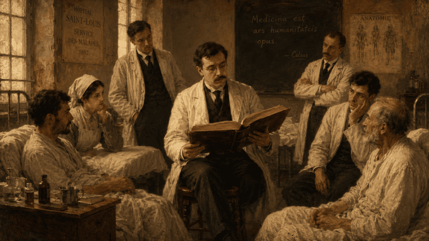
A doctor reads from a large medical book in an early 20th-century hospital ward, surrounded by attentive patients and fellow physicians.

Narrative Medicine: Close Reading, Clinical Empathy, and the Art of Listening to Patients

Posted on August 8, 2026August 16, 2026 by Michele Danilo Pierri

1. Introduction: Why Narrative Medicine Matters Now

In an era defined by algorithmic diagnostics, electronic health records, and the quantification of care, medicine faces a paradox: as its technical capacity has expanded to unprecedented heights, the therapeutic relationship — the conversation between patient and clinician — has frequently contracted. Patients report feeling unheard. Physicians report feeling burned out. Diagnostic errors persist not from lack of data but from failures of attention. Against this backdrop, narrative medicine has emerged not as a romantic retreat from science but as a rigorous, evidence-informed discipline that restores the human story to its proper place at the centre of clinical practice.

The term “narrative medicine” names a discipline that — in the formulation of its chief architect, Rita Charon — is “medicine practised with narrative competence.” That competence entails the ability to recognise, absorb, interpret, and be moved by the stories patients tell of their illnesses; to understand illness as an event in someone’s life trajectory; and to reflect, with critical precision, on the stories clinicians themselves construct. Far from being optional ornamentation on a scientific core, narrative competence turns out to be implicated in the accuracy of diagnosis, the depth of empathy, and the resilience of practitioners themselves.

This interpretive reading of the body is not a modern invention. Long before clinical semiotics was formalised, literature had already practised it: Dante’s Inferno, for instance, reads the damned as a precise catalogue of disease, transforming the poet’s gaze into something remarkably close to a clinician’s.

This post offers a comprehensive introduction to narrative medicine clinical practice for clinicians, researchers, and medical educators with an interest in the intersections of data, science, and the human dimension of healthcare. We move from historical origins through theoretical foundations, examine the evidence base, read canonical literary and artistic works through a narrative medicine lens, distinguish the field from the broader territory of medical humanities, and close with practical tools clinicians can adopt immediately.

2. Origins: Rita Charon and the Columbia Programme

The story of narrative medicine as a formal discipline begins with an internist and literary scholar named Rita Charon. Charon arrived at Columbia University’s College of Physicians and Surgeons in the 1990s carrying two doctoral degrees — one in medicine, one in English literature — and a persistent intuition that something in the medical encounter was being systematically missed. Her concern was not sentimental: it was epistemological. She believed that the modes of attention and interpretation trained by literary study were directly transferable to clinical encounters, and that physicians who lacked those modes were not merely less humane but less accurate.

In 2000, Charon published a landmark paper in JAMA titled “Narrative Medicine: A Model for Empathy, Reflection, Profession, and Trust,” articulating for the first time a coherent programme. Three years later she founded the Programme in Narrative Medicine at Columbia, the first of its kind. The programme trained physicians, nurses, social workers, and chaplains in close reading, reflective writing, and the analysis of narrative structure. It drew its curriculum from literary theory — particularly from the work of Mikhail Bakhtin on dialogism and from narratologists such as Gérard Genette — and from medical ethics and philosophy.

What distinguished Charon’s project from earlier work in literature and medicine (which had been practised informally for decades) was its insistence on rigour. Narrative medicine was not bibliotherapy — the therapeutic use of reading. It was a discipline with defined methods, teachable skills, and, crucially, outcomes that could be measured. The programme has since trained hundreds of healthcare professionals and spawned postgraduate certificates, master’s degrees, and doctoral programmes at Columbia and at affiliated institutions worldwide.

The intellectual genealogy of the field is worth tracing briefly. Charon drew on Arthur Kleinman’s distinction between disease (the biological pathology) and illness (the patient’s experienced suffering), a distinction Kleinman elaborated in The Illness Narratives (1988). She drew on Eric Cassell’s The Nature of Suffering (1991), which argued that medicine’s failure to engage with personhood — with biography, with meaning — caused suffering beyond the biological. And she drew on phenomenological philosophy, particularly Edmund Husserl and Maurice Merleau-Ponty, which insisted that bodily experience was the irreducible foundation of human knowledge. Together, these sources supported the central claim: that the patient’s narrative is not background information but primary clinical data.

3. The Four Core Elements: Attention, Representation, Affiliation, Action

Charon and her colleagues articulate narrative medicine around four cardinal concepts: attention, representation, affiliation, and action. These are not sequential steps but mutually reinforcing capacities, each of which can be cultivated through practice.

Attention

Attention is the disciplined act of receiving — of opening oneself to the full complexity of what a patient presents. In literary close reading, attention means noticing what a text does formally: its rhythm, its silences, its metaphors, its shifts in tense or person. In the clinical encounter, it means noticing not just the content of what a patient says but the form in which they say it: the hesitation before naming a symptom, the passive construction used when describing a traumatic event, the moment when the patient’s gaze drops away. Attention in this sense is active and trained, not passive and instinctive. It requires the clinician to suspend premature closure — the drive to pattern-match and categorise — and to remain, for longer than is comfortable, in a state of receptive uncertainty.

Representation

Representation is the act of making what has been attended to into an external form — a written note, a narrative account, a parallel chart (discussed below). For Charon, the act of writing is not merely documentation but transformation: in writing about a patient encounter, the clinician moves from raw perception to structured meaning, and in doing so discovers what they noticed and what they missed, what moved them and what they avoided. Representation is where the work of close reading rejoins the work of clinical documentation, and where the parallel chart becomes a tool of both self-knowledge and quality improvement.

Affiliation

Affiliation is the outcome of sustained attention and honest representation: a genuine sense of connection with the patient, grounded not in sentimentality but in the recognition that the patient’s suffering is particular, not generic. In Charon’s formulation, affiliation is the emotional and ethical correlate of narrative competence. It is what prevents the clinician from treating the patient as a case and insists on treating them as a person. Crucially, affiliation is not the same as identification: the clinician does not need to have had the same experience as the patient to be affiliated with them. What is required is the imaginative capacity to understand — not fully, but seriously — a life that is not one’s own.

Action

Action is the translation of narrative competence into changed clinical behaviour: a different question asked, a diagnosis reconsidered, a conversation opened that had been avoided, a care plan altered in response to what the patient has actually said rather than what the clinician expected to hear. Action is the test of narrative medicine’s claim to clinical utility. If close reading and reflective writing produce only private insight, they remain valuable but limited. Their full potential is realised when they alter the clinician’s behaviour in ways that improve the quality of care.

4. The Evidence Base: Empathy, Burnout, and Diagnostic Accuracy

Sceptics sometimes characterise narrative medicine as an appealing idea in search of evidence. The evidence, while still accumulating, is more substantial than critics acknowledge.

On empathy, a 2001 study by Halpern demonstrated that emotional attunement — closely related to narrative competence — was associated with improved patient outcomes across multiple measures. More directly, a 2011 randomised controlled trial by Winkel and colleagues, published in Patient Education and Counseling, found that narrative medicine training significantly improved empathy scores in medical students compared to controls, with effects sustained at six-month follow-up. DasGupta and Charon’s own work has consistently shown improvements in perspective-taking and tolerance of ambiguity following narrative medicine seminars.

On clinician burnout, the evidence is suggestive and important. Burnout in medicine is partly a consequence of the erosion of meaning — the sense that clinical work has been reduced to procedure and throughput. Narrative medicine addresses this directly by restoring the clinician’s sense of the meaning of their work. Studies at Columbia and at Thomas Jefferson University have shown that narrative medicine workshops reduce emotional exhaustion and increase personal accomplishment scores on the Maslach Burnout Inventory. A 2019 systematic review by Milota, van Thiel, and van Delden, published in Medical Teacher, found consistent positive effects on reflective capacity and on measures of professional identity across diverse narrative medicine curricula.

On diagnostic accuracy, the connection is more inferential but theoretically compelling. Jerome Groopman’s How Doctors Think (2007) — discussed in detail below — documents how cognitive biases, including premature closure and anchoring, account for a substantial proportion of diagnostic errors. Narrative competence addresses these biases directly: by training clinicians to maintain attention to disconfirming detail and to remain open to revision, it targets the cognitive habits that make errors most likely. Research by Smith and colleagues has shown that physicians who score higher on measures of narrative competence are more likely to elicit complete patient histories and to identify psychosocial factors relevant to diagnosis.

These findings should be interpreted carefully: narrative medicine research faces the general challenges of educational intervention studies, including difficulty blinding, variability in implementation, and the problem of measuring outcomes that unfold over years rather than weeks. But the direction of evidence consistently supports the field’s core claims, and the methodological maturity of the literature has grown considerably since the early 2000s.

5. Narrative Medicine Through Literary and Artistic Works

Narrative medicine gains much of its intellectual depth from sustained engagement with literary and artistic works that explore illness, suffering, and the medical encounter. Six works in particular illuminate different dimensions of narrative medicine clinical practice and have become central to its pedagogical canon.

Leo Tolstoy, The Death of Ivan Ilyich (1886)

Tolstoy’s novella remains the most powerful literary exploration of what Charon calls the “narrative situation of illness.” Ivan Ilyich Golovin, a successful judge, develops an illness that his physicians never diagnose with confidence and that none of his colleagues or family members are able to acknowledge honestly. The novella’s central indictment is not of medicine’s technical failures but of its narrative ones: the physicians who attend Ivan Ilyich are interested in the disease, not the man; they deliver verdicts in the language of probability and prognosis while remaining utterly silent on the questions that actually consume their patient — why is this happening to me, and what does it mean?

The key passage for narrative medicine is Ivan Ilyich’s recognition that “what he longed for most was to be pitied and wept over as a sick child is caressed and comforted.” The longing is not for cure but for witness — for the acknowledgement that his suffering is real and that it matters to someone. Gerasim, the peasant servant who alone is straightforward with Ivan Ilyich, represents the therapeutic power of honest attention. He does not diagnose or treat; he simply holds the dying man’s legs through the night because it eases the pain. In doing so he performs, intuitively, what narrative medicine formalises as affiliation. Tolstoy’s novella stands as a reminder that technical excellence and narrative failure are not mutually exclusive — and that the second can hollow out the first.

This indictment takes different forms across literary traditions. Where Tolstoy’s physicians fail through scientific detachment, Proust’s celebrated Dr Cottard fails through vanity: a socially ambitious, at times absurd figure whose diagnostic reputation masks a striking poverty of human attention — a portrait explored elsewhere on this site.”

Virginia Woolf, On Being Ill (1926)

Woolf’s essay is a masterpiece of illness phenomenology, written from the inside. Her central provocation is a question: why, given that illness is among the most universal of human experiences, has it generated so little literature? “Considering how common illness is, how tremendous the spiritual change that it brings, how astonishing, when the lights of health go down, the undiscovered countries that are then disclosed, what wastes and deserts of the soul a slight attack of influenza brings to view” — why has this territory been left unmapped?

For narrative medicine, Woolf’s essay performs two related functions. First, it gives language to experiences that patients typically lack words for: the altered temporality of illness, the estrangement from the healthy body, the strange clarity of perception that fever sometimes brings. Second, it implicitly diagnoses the physician’s epistemological problem: if the clinician has not attended to the literature of illness, they have no map for the territory their patients inhabit. Woolf’s essay is, in this sense, a corrective to professional habituation — a reminder that illness is not a deviation from the norm of health but a distinct, complex country with its own geography, and that the physician who has never ventured into that country, even through the proxy of literature, is navigating it blind.

Franz Kafka, The Metamorphosis (1915)

Gregor Samsa’s transformation into a giant insect is one of literature’s most persistent metaphors for the experience of chronic illness. What Kafka renders with extraordinary precision is not the biology of transformation but its social consequences: the withdrawal of recognition, the restructuring of family relationships around the sick member’s incapacity, the gradual erosion of the ill person’s subjectivity in the eyes of those around them. Gregor’s family members pass through stages — shock, accommodation, resentment, guilt — that closely parallel the documented emotional trajectories of families confronting chronic or terminal illness.

For clinical practice, The Metamorphosis is a study in what Arthur Frank has called the failure of the “restitution narrative”: when cure is not available, the social structures that organise illness break down, and both patient and family are left in a narrative void. The story is a reminder that the patient’s illness story is always also a family story — and that the clinician who attends only to the individual patient misses the broader systemic context in which that patient’s suffering unfolds. Reading Kafka carefully can help clinicians recognise the systemic dimensions of their patients’ crises that a disease-centred history will never surface.

The same logic of somatised suffering runs through contemporary fiction as well: Murakami’s bodies, where insomnia, anorexia and the amputated shadow stand in for wounds that never reach clinical language.

Anton Chekhov: The Physician-Writer

Chekhov occupies a unique position in the narrative medicine canon because he wrote from both sides of the consultation room. Trained as a physician and practising throughout his adult life — dying of tuberculosis at forty-four — Chekhov brought to his fiction a clinical precision that was inseparable from his literary technique. His stories — “Ward No. 6,” “A Boring Story,” “The Bishop,” among many others — are studies in observation and restraint, in what he famously described as writing “without commentary.”

For narrative medicine, Chekhov’s method is itself an object of instruction. His refusal to judge, his insistence on showing rather than telling, his attention to the gap between what characters say and what they feel — these are literary virtues that translate directly into clinical ones. “Ward No. 6” in particular, with its portrayal of a physician who gradually identifies with his patient to the point of becoming one himself, raises the problem of affiliation taken to pathological extremes. The clinician’s challenge is to be moved without being overwhelmed; to be present without losing the reflective distance necessary for good judgment. Chekhov dramatises this challenge with a clarity that no clinical textbook has matched. His dual identity — as physician and as writer — also makes him the emblematic figure for the kind of integrative attention that narrative medicine seeks to cultivate.

Oliver Sacks: The Neurological Case History as Literature

Oliver Sacks represents a different kind of intervention: the physician who borrows the tools of literary narrative to transform the case history into a form of humanistic inquiry. In The Man Who Mistook His Wife for a Hat (1985), Awakenings (1973), and his later autobiographical work, Sacks consistently positioned the patient not as a bundle of symptoms but as a person navigating the meaning of a profoundly altered existence.

Sacks was explicit about his method. He described himself as a “clinical neurologist and romantic naturalist,” and his prose style — dense with literary and cultural allusion, attentive to the phenomenology of experience, deliberately unhurried — was a formal argument for a different kind of medical attention. For narrative medicine, Sacks’s most important contribution may be his insistence on what he called the “existential dimension” of neurological illness: that diseases of the brain are always simultaneously diseases of the self, and that understanding them requires attending to the patient’s experience of selfhood rather than merely to the pathology of the underlying neural mechanisms. His case histories enact precisely the movement from representation to affiliation that Charon’s framework prescribes. They also demonstrate, with unusual clarity, that rigorous clinical observation and humanistic narrative are not competing but complementary modes of knowledge.

Jerome Groopman, How Doctors Think (2007)

Groopman’s work occupies a different register — more journalistic than literary, more oriented toward cognitive science than phenomenology — but it connects powerfully to narrative medicine’s concerns. Through a series of extended case studies, Groopman demonstrates how physicians’ thinking goes wrong: premature closure (accepting the first plausible diagnosis and stopping), anchoring (over-weighting the initial impression), availability bias (over-diagnosing conditions recently prominent in the physician’s experience), and attribution error (assigning symptoms to a pre-existing condition without adequate investigation).

What is striking from a narrative medicine perspective is that virtually all the cognitive errors Groopman documents are failures of attention to the patient’s narrative. The physician who anchors closes off the patient’s story before it is complete; the physician who commits attribution error fails to hear the plot twist that contradicts the working hypothesis. Groopman’s implicit prescription — slow down, listen more carefully, ask open questions — is indistinguishable from narrative medicine’s explicit training programme. Reading How Doctors Think alongside Charon’s theoretical work reveals that cognitive science and narrative theory, approached from different angles, converge on the same clinical insight: the quality of a physician’s listening determines the quality of their diagnosis.

Visual Art: Rembrandt and the Anatomy Lesson

Narrative medicine extends beyond literature into visual art, and few works repay close reading as richly as Rembrandt van Rijn’s The Anatomy Lesson of Dr Nicolaes Tulp (1632). The painting depicts a public dissection in Amsterdam: Dr Tulp demonstrates the musculature of the forearm of a recently executed criminal to seven observers. The composition is remarkable for its distribution of attention: six of the seven observers look not at the body being dissected but at the viewer, the book, or each other; only Dr Tulp gazes at the cadaver and at his own demonstrating hand.

For narrative medicine, the painting raises the question that Charon considers foundational: who is the patient in this scene? The cadaver — Adriaan Adriaanszoon, also known as “Aris Kindt” — is the object of scientific attention, but he is also a person with a biography, a story that ended violently on a scaffold. The anatomy lesson performs, literally and symbolically, the gesture that narrative medicine seeks to reverse: the body reduced to object, the story suppressed in the service of knowledge. Reading the painting closely — attending to the cadaver’s face, to the pallor that Rembrandt renders with such precision, to the space between the clinical act and the human life it consumes — is itself an exercise in the kind of attention narrative medicine cultivates. Using visual art in teaching narrative medicine has the additional advantage of making the interpretive process visible: students who disagree about what a painting means are enacting precisely the dialogic, multiple-perspective engagement that Bakhtin theorised and that clinical encounters require.

6. Narrative Medicine vs Medical Humanities: Related but Distinct

Narrative medicine is sometimes treated as synonymous with medical humanities, but the distinction matters — both intellectually and for institutional purposes. Medical humanities is the broader field: it encompasses history of medicine, ethics, philosophy, sociology, anthropology, literature, and visual arts, and its goals range from cultural critique to professional formation to the improvement of clinical practice. It is a multi-disciplinary domain united by the conviction that humanistic inquiry can enrich medical education and practice.

Narrative medicine is a discipline within this broader field, but distinguished by its specificity of method and its direct claim on clinical practice. Where medical humanities may ask “what does the history of the asylum tell us about the social construction of mental illness?”, narrative medicine asks “how does close reading this poem about dementia change the way you listen to your patient with Alzheimer’s disease in the clinic this afternoon?” The difference is not one of value but of proximate aim: medical humanities is primarily oriented toward understanding; narrative medicine is primarily oriented toward changing clinical behaviour.

The methodological core of narrative medicine — close reading, reflective writing, the analysis of narrative structure — is borrowed from literary studies in a way that is more precisely specified and more pedagogically worked-out than most medical humanities programmes. And narrative medicine’s claim to clinical utility is stronger: it is not primarily an enrichment activity but a skills training programme, one that can be evaluated against clinical outcomes. Charon has consistently resisted the assimilation of narrative medicine into the looser category of medical humanities precisely because that assimilation tends to dilute the methodological rigour that makes the field distinctive.

That said, the fields are deeply complementary. The historical depth that medical humanities brings — the understanding of how concepts of disease, body, and care have varied across cultures and periods — provides essential context for the narrative medicine practitioner. And narrative medicine’s clinical focus gives medical humanities a practical anchor that helps justify its place in crowded medical curricula. The two fields are best understood as nested: narrative medicine is a rigorously specified method within the expansive territory that medical humanities claims as its domain.

7. How Clinicians Can Practice It: Tools for Everyday Use

Narrative medicine is not confined to graduate programmes or academic hospitals. Its core practices can be adopted by any clinician willing to invest time and reflective attention. Three tools are particularly accessible and evidence-supported.

The Parallel Chart

The parallel chart is perhaps narrative medicine’s most distinctive clinical tool. Alongside the official medical record — formal, structured, written for institutional purposes — the parallel chart is a private document in which the clinician records their own narrative of the encounter: what they noticed that they could not record in the EMR, what the patient said that moved them, what they found difficult, what they remain uncertain about. The parallel chart is not a diary; it is a disciplined reflective exercise, and its format — close attention to detail, narrative structure, honest accounting of emotional response — mirrors the practices of close reading.

The clinical purpose is manifold. It preserves information that institutional documentation suppresses (the patient’s exact words, the affective texture of the encounter) but that may be clinically relevant later. It provides a space for the clinician to notice and process their own responses, reducing the risk that unprocessed emotion will distort future clinical judgment. And it serves, over time, as a record of the clinician’s developing narrative competence — a log of the quality of their attention that no EMR can provide.

Close Reading in Clinical Teaching

Close reading as a pedagogical method is directly applicable to clinical education. A narrative medicine seminar typically begins with a short text — a poem, a short story excerpt, a painting — presented to the group without biographical or contextual framing. Participants are asked not to summarise or contextualise but to attend closely to the text’s specific features: its structure, its imagery, its voice, its silences. Discussion unfolds through careful attention to what the text actually does, rather than what one expects it to do.

This practice of disciplined attention is then transferred to the clinical context: the patient’s story, the physical examination, the clinical note become texts to be read with the same precision. In medical schools that have integrated narrative medicine — Columbia, Harvard, UC San Francisco, King’s College London among them — close reading sessions are included in the formal curriculum alongside biomedical science. Evaluations consistently show improvements in students’ reported empathy, their tolerance of ambiguity, and their willingness to engage with patients’ psychosocial contexts.

Reflective Writing

Reflective writing in narrative medicine differs from the general reflective practice advocated in medical education in its attention to craft. Where standard reflective practice asks “what happened, what did I feel, what would I do differently?”, narrative medicine reflective writing asks clinicians to attend to the formal dimension of their own narratives: whose perspective is privileged, what is left out, what metaphors are used, what the structure of the account reveals about the writer’s assumptions.

Charon recommends a specific exercise called the “narrative of the clinical encounter”: immediately after seeing a patient, the clinician writes a brief account of the encounter in whatever form emerges naturally. The account is then read aloud in a small group (in training settings) or analysed privately, with attention to the narrative choices the writer made. Over time, this practice develops what Charon calls “narrative humility” — an awareness of the partiality of one’s own perspective and the inevitability of narrative construction in clinical knowledge. It is a practice with no expensive equipment requirement and no institutional permission needed: it requires only a few minutes and the willingness to be honest with oneself.

Grand Rounds and Case Conferences

Narrative medicine’s methods can also be integrated into existing institutional structures without requiring a dedicated curriculum. Grand rounds presentations can be expanded to include the patient’s narrative alongside the clinical history; case conferences can include time for reflective discussion of the interpersonal and affective dimensions of a case, not merely its diagnostic and therapeutic aspects. These are modest structural changes, but when implemented consistently they shift the culture of clinical education toward the values of attention, representation, and affiliation — making narrative competence a recognised professional virtue rather than a private eccentricity.

8. Conclusion: Listening as Clinical Practice

The argument of narrative medicine is, at its core, straightforward: the stories patients tell are data, and the capacity to receive and interpret those stories is a clinical skill that can and must be trained. In an era when medicine is under pressure — from technology, from system constraints, from the burden of documentation — this argument can seem naively humanistic. In fact, it is hard-headedly practical. The physician who listens well diagnoses more accurately. The clinician who writes reflectively burns out less quickly. The healthcare system that takes patient narratives seriously makes fewer errors and generates more trust.

This post is part of a broader investigation, on this site, into the intersections of data science, artificial intelligence, and medical humanities. In previous posts we have explored how quantitative methods can illuminate questions of human significance, and how the humanities offer resources for thinking about the limits of quantification. Narrative medicine sits precisely at this intersection: it uses the rigorous methods of literary analysis to generate clinical knowledge that quantitative methods alone cannot produce. It is neither anti-scientific nor anti-technological; it is, rather, a reminder that the most advanced clinical tool remains the disciplined human ear.

For clinicians reading this, the invitation is immediate and concrete: choose one patient today, listen to their opening words without interrupting, notice the form of what they say and not merely its content, and write a paragraph — not in the EMR but privately — about what you noticed. That paragraph is the beginning of a parallel chart, and the beginning of a practice that the evidence suggests will make you a better physician and a more resilient one.

Ivan Ilyich, the judge who died alone in Tolstoy’s novella, did not recover. But he died, in Tolstoy’s rendering, with something that had been absent throughout his illness: the experience of being genuinely seen. That experience — of being a person rather than a case, of one’s suffering mattering to another human being — is not a luxury at the margins of clinical care. It is, narrative medicine argues, very close to its centre.

References and Further Reading

Cassell, E. J. (1991). The Nature of Suffering and the Goals of Medicine. Oxford University Press.
Charon, R. (2001). “Narrative Medicine: A Model for Empathy, Reflection, Profession, and Trust.” JAMA, 286(15), 1897–1902.
Charon, R. (2006). Narrative Medicine: Honoring the Stories of Illness. Oxford University Press.
Frank, A. W. (1995). The Wounded Storyteller: Body, Illness, and Ethics. University of Chicago Press.
Groopman, J. (2007). How Doctors Think. Houghton Mifflin.
Halpern, J. (2001). From Detached Concern to Empathy: Humanizing Medical Practice. Oxford University Press.
Kleinman, A. (1988). The Illness Narratives: Suffering, Healing, and the Human Condition. Basic Books.
Milota, M. M., van Thiel, G. J. M. W., & van Delden, J. J. M. (2019). “Narrative medicine as a medical education tool: A systematic review.” Medical Teacher, 41(7), 802–810.
Sacks, O. (1985). The Man Who Mistook His Wife for a Hat. Summit Books.
Tolstoy, L. (1886). The Death of Ivan Ilyich. Trans. R. Pevear & L. Volokhonsky. Vintage.
Woolf, V. (1926). On Being Ill. Hogarth Press.

distressed early 20th-century doctor struggles to inject an enormous syringe labeled “Llama 3.1 405B Parameters” into a tiny desktop PC

The Model Runs, the User Waits: The Paradox of Large Local LLMs

Posted on August 3, 2026August 16, 2026 by Michele Danilo Pierri

Hunting for the largest language model you can run on a personal computer has turned into a discipline of its own. Forums, repositories and social feeds circulate configurations that load models of 70, 120, even several hundred billion parameters, using consumer GPUs, generous amounts of system RAM and increasingly aggressive quantisation.

The results are frequently impressive as engineering. A model that would need well over a hundred gigabytes at FP16 precision can be compressed, spread across GPU and system memory, and finally brought up on a workstation that is not out of reach.

There remains a less spectacular question, and a far more consequential one:

If the model produces one or two tokens per second, can we honestly call it usable?

Being able to load a model and being able to work with it are two different achievements. The first is a memory problem. The second involves latency, bandwidth, quality, context, power draw and human time.

The distinction matters especially in healthcare. Local processing can offer real advantages for certain workflows — those touching sensitive data, operational continuity, or integration with internal systems. But precisely because the setting is critical, a solution cannot be judged by the number of parameters it manages to load. It has to be reliable, governable, and fast enough to slot into workflows as they actually run.

“It runs locally” is not a benchmark

When someone describes a local installation, the phrase “the model runs” can mean any of several quite different things:

the process started without exhausting memory;
the model produced at least one reply;
generation happens at an acceptable speed;
the system stays fast with long documents;
quality is sufficient for the intended task;
several users can work with it at once;
the output arrives within the operational window required.

Demonstrations published online usually verify only the first two.

Hence a misunderstanding: getting the model to start is treated as proof that it is useful. But an interactive system is not judged on whether it eventually completes a computation. It is judged on how long it takes to hand back something you can use.

Assessing a local LLM takes at least four measurements.

Time to first token, or TTFT. How long passes between sending the request and the start of the reply.

Prompt processing. How quickly the system chews through the incoming text. This becomes decisive when the prompt carries a clinical record, a document, a transcript, or a set of passages retrieved through a RAG pipeline.

Generation speed. The number of tokens produced per second during the reply.

Time to complete response. The metric closest to what the user perceives, and to the operational value of the system.

A model can generate at a decent clip yet take a long time to digest a lengthy document. Or it can start replying almost immediately and then spend several minutes finishing a long chain of reasoning. Tokens per second alone do not tell the whole story — but ignoring them means overlooking one of the main reasons local deployments end up unusable.

Why generation is so sensitive to memory

Inference in an autoregressive model has two main phases.

During prefill, the model processes the prompt and builds the representations it needs to begin answering. This work parallelises well and is typically limited by compute capacity.

During decode, tokens come out one at a time. Each new token depends on the ones before it. In this phase, how fast weights, cache and activations can be read from memory usually matters more than the GPU’s theoretical arithmetic throughput. Interactive generation, in other words, tends to be a memory-bound workload [1].

That explains why VRAM is not merely a place to park the model. It is also very high bandwidth memory.

When a substantial portion of the model is moved into system RAM, the capacity problem may be solved, but the system now has to route part of the work through a far slower memory subsystem. It is not enough for the model to “fit” into the sum of RAM and VRAM: what counts is where its components sit during each generation step.

Quantisation: less memory, but not for free

The most widespread technique for running large LLMs locally is quantisation. Weights, normally held as 16-bit numbers or larger, are converted into reduced-precision formats.

As a first approximation, a 70-billion-parameter model needs roughly 140 GB for weights alone at FP16. Quantising to 8 bits can halve that footprint; 4-bit can cut it to about a quarter, before you add metadata, buffers and cache on top [2].

Four-bit quantisation is often held up as the sweet spot. A good deal of published work shows that, with the right techniques, it preserves much of the original model’s quality. That observation does not license treating every format or every compression level as equivalent.

As you push down towards 3 or 2 bits:

the risk of distorting the model’s output distributions rises;
some capabilities degrade unevenly;
available context may shrink;
outcomes depend heavily on calibration and on the format chosen;
apparent coherence and actual quality can drift apart.

The llama.cpp project uses perplexity, KL divergence, probability shifts and top-token agreement rate to quantify the loss introduced by quantisation [3]. The point deserves emphasis: confirming that a model still produces grammatically plausible text says nothing about whether it retains the original’s capabilities.

Quantisation also affects speed in ways that are not uniform. A more compact format reduces the volume of data to be read, but it demands kernels and runtimes able to process it efficiently. Compression that looks advantageous on paper does not automatically translate into a speed-up on arbitrary hardware.

ExLlamaV2, to take one example, showed that a Llama 2 70B at roughly 2.5 bits can run on a 24 GB GPU at speeds in the tens of tokens per second [4]. A notable result — but obtained with extreme quantisation, an optimised runtime and a constrained context. It is not a general rule for any 70B, nor does it show that quality and performance match the original.

So the right question is not “how far can I compress this model?” but:

What is the highest level of compression compatible with the quality my use case demands?

In healthcare that question has to be asked task by task. A quantisation that works perfectly well for sorting administrative documents may prove inadequate for pulling out rare clinical findings or interpreting complex relationships.

CPU offload: the model fits, the speed leaves

When VRAM runs short, runtimes such as llama.cpp let you keep some layers on the GPU and the rest in system RAM [5]. This hybrid CPU–GPU inference makes it possible to run models that the available hardware could not otherwise host.

It is also the technique that exposes the gap between feasibility and usability most plainly.

Discussions in the LocalLLaMA community contain plenty of examples of 70B models running on a single 24 GB GPU with the remaining weights in RAM. Reported performance varies with the model, the quantisation, the processor, the memory, the context and the number of layers pinned to the GPU.

In one case, a system with an RTX 4090 and 64 GB of DDR5 generated around 1.2 tokens per second on a 70B Q5 partially resident in RAM. In the same thread, a far more aggressive quantisation — small enough to sit almost entirely on the GPU — reached roughly 10 tokens per second [6].

These figures are anecdotal and should not be read as scientific benchmarks. They are useful all the same for describing the phenomenon: having a very fast GPU does not prevent the slowdown once a meaningful share of the processing falls back on system memory.

Another test, with a 14B model, recorded around 70 tokens per second as long as model and context stayed inside VRAM. Once capacity was exceeded, RAM and CPU stepped in and generation dropped to about 19 tokens per second — even though most of the load was still nominally assigned to the GPU [7].

Offload remains valuable for:

batch processes with no interactive requirement;
experimentation and occasional evaluation;
overnight generation runs;
environments where capacity matters more than latency;
models used rarely, as an escalation tier.

It is far less convincing for chatbots, voice assistants, code completion, and clinical workflows where a professional has to wait for the output before carrying on.

Context consumes memory and time

Weights are not the only thing occupying memory. During inference the system maintains a KV cache holding information about tokens already processed. Its size grows with context length, batch size and model architecture.

NVIDIA estimates that for Llama 3 70B, a 128,000-token window can require around 40 GB of KV cache for a single user [8].

The theoretical ability to accept very long contexts is therefore no guarantee that those contexts are usable on the system in front of you. As context grows, you may see:

less VRAM left for the weights;
part of the load shifting into RAM;
longer time to first token;
attention slowing down;
fewer concurrent users supported;
out-of-memory failures.

KV cache quantisation, Flash Attention, prompt caching, sliding windows and selective context reduction can all take the edge off. But the most effective improvement is usually the least glamorous one: stop sending the model information it does not need.

For a healthcare application, that means designing extraction, retrieval and document segmentation with care, rather than leaning indiscriminately on ever-larger context windows.

How many tokens per second do you actually need?

There is no universal threshold. A batch procedure can be useful at one token per second; a voice assistant can feel broken at ten. For a single user, though, a rough scale is workable.

Generation speed	Indicative experience
Under 2 tokens/s	Technical demo or batch process
2–5 tokens/s	Occasional use with obvious waiting
5–10 tokens/s	Slow but workable interaction
10–20 tokens/s	Conversation generally practicable
20–50 tokens/s	Fluid experience
Above 50 tokens/s	Perceived as very fast

NVIDIA cites 5 tokens per second as an example below typical reading speed, and 50 tokens per second as an example of an excellent experience [9]. These are indications, not clinical or universal thresholds.

To see what the number means in practice, take a 1,000-token generation:

at 2 tokens/s it takes about 8 minutes 20 seconds;
at 5 tokens/s, about 3 minutes 20 seconds;
at 10 tokens/s, about 1 minute 40 seconds;
at 50 tokens/s, about 20 seconds.

With reasoning models the problem can be sharper still. If the system emits thousands of intermediate tokens, a speed that would be acceptable for a short answer can produce latencies of several minutes.

In a healthcare workflow the effect is not merely perceptual. Excessive latency can push the user to abandon the tool, run tasks in parallel, lose the operational thread, or fall back on alternative procedures that nobody is governing.

Unified memory, multiple GPUs and speculative decoding

Other strategies exist for getting past the single-GPU ceiling.

Unified memory systems let CPU and GPU draw on a common pool. This softens the rigid split between RAM and VRAM and makes larger models loadable. It does not remove the bandwidth constraint: capacity grows, but speed still depends on architecture and runtime.

Using multiple GPUs allows weights and compute to be distributed. The benefit hinges on how fast the cards can talk to each other. Technologies such as NVLink and NVSwitch exist precisely so the interconnect does not become the new bottleneck [9]. Two consumer GPUs joined only over PCIe are not automatically equivalent to a single GPU with the same total memory.

Speculative decoding takes a different route: a smaller model proposes several tokens, which the main model then verifies in a block. When proposals are accepted often enough, the technique speeds up generation without altering the target model’s distribution. llama.cpp supports both draft models and n-gram-based methods [10].

A promising optimisation, then, though not a universal answer. It costs additional memory for the draft model, and it is unlikely to turn an offload-dominated configuration into a genuinely fast one.

The hidden cost of “free and local”

Local execution is often set against cloud APIs on the basis of per-token cost alone. That comparison is incomplete.

A large local model also brings:

hardware purchase and depreciation;
energy consumption;
cooling and noise;
maintenance of drivers, runtimes and quantisations;
time spent on testing and updates;
slower iteration;
unused capacity during idle periods;
the cost of the time spent waiting for answers.

In a healthcare organisation, governance costs join the list:

access control;
environment segregation;
logging and audit;
version management;
performance verification;
quality assessment;
error monitoring;
operational continuity.

Local does not automatically mean secure, compliant or governed. It means the organisation retains greater control over the execution environment. That control still has to be exercised through appropriate architecture and procedures.

Why local still matters in healthcare

Health data falls within the categories of personal data given special protection under the European framework. The European Data Protection Board has also reiterated that the development and use of AI models must be assessed against GDPR principles, including effective anonymity, lawful basis and the processing of personal data [11].

The European Health Data Space Regulation, for its part, builds a framework for access, control, exchange and secure reuse of electronic health data. It entered into force on 26 March 2025, with its provisions applying progressively [12].

None of this implies that every piece of healthcare processing has to happen locally. Compliance depends on purpose, lawful basis, roles, contracts, technical measures, localisation, minimisation and a good many other factors.

There are nevertheless cases where processing kept local, or inside the organisation’s own infrastructure, offers concrete advantages:

classifying documents containing identifying data;
extracting fields from reports and forms;
semantic indexing of internal archives;
preliminary anonymisation or pseudonymisation;
searching confidential procedures and documentation;
transcription and normalisation within authorised environments;
activities that must continue without external connectivity;
applications where sending content to a remote service is not contemplated by the governance model.

For tasks of this kind, a small, fast, specialised model can deliver more value than a very large but sluggish one.

Parameter count should not stand in for validation. Within a well-bounded process, a smaller model can be evaluated against a representative dataset, constrained to a structured output format, and wrapped in a pipeline with deterministic checks.

Hybrid architecture as a design choice

The opposition between “all local” and “all cloud” is often artificial. A hybrid solution can assign each activity to whichever environment suits it.

One possible flow:

local processing of identifying data;
classification of the request with a compact model;
local execution of simple or sensitive tasks;
removal or transformation of unnecessary data;
controlled escalation to a more capable model when the task warrants it;
local validation and logging of the outcome.

The local model can handle:

routing;
structured extraction;
normalisation;
short summaries;
document search;
template application;
preliminary checks;
protection or removal of identifiers.

The remote or centralised model can be reserved for:

complex reasoning;
exceptionally long documents;
ambiguous requests;
infrequent problems;
second-line verification;
tasks where the local model does not reach the required confidence.

Escalation should not fire automatically and indiscriminately. It needs to be governed through rules, data classification, consent or authorisation where required, content minimisation, and a choice of providers and configurations consistent with the organisational framework.

Seen this way, the local model is not an impoverished version of the cloud model. It is a different component, tuned for privacy, latency, control and specialisation. The larger model becomes a resource to be drawn on selectively, not the obligatory engine behind every request.

From model-first to task-first

The race to run the biggest possible LLM locally usually starts from a model-first posture: pick the model, then look for a way to bend the hardware around it.

A useful architecture should start from the task:

What accuracy is required?
What latency is acceptable?
What data may the model see?
How much context is really needed?
Is the process interactive or batch?
What happens when the model gets it wrong?
Is there a human in the loop?
When is escalation permitted?
What level of availability is required?

Only after these questions does it make sense to choose size, quantisation, runtime and placement.

The headline metric is not the maximum number of parameters you can load. It is the smallest system capable of completing the task correctly within the constraints you have set.

Conclusion: better small and functional

Running a model with tens of billions of parameters locally, on consumer hardware, is a fascinating technical achievement. Quantisation, offload, unified memory, multi-GPU distribution and speculative decoding have vastly expanded what can be done outside the data centre.

Technical possibility is not the same as usefulness.

A model generating one or two tokens per second may suit a batch process, an experiment, or a task you run rarely. It should not be presented as an interactive solution merely because it manages to produce an answer.

In healthcare, local retains strategic value. It can reduce data exposure, support controlled processes and provide operational independence. For that value to materialise, though, the system has to be fast enough, validated on the task, and embedded in adequate governance.

Real success is not seeing a 70- or 120-billion-parameter model appear in the process list. It is getting an answer good enough, quickly enough, that you can carry on working.

Better small and functional than large and unusable.

And when the task genuinely calls for more capability, the rational answer is not to wait longer: it is to adopt a hybrid architecture.

References

NVIDIA, “Mastering LLM Techniques: Inference Optimization”, 2023. Online.
Hugging Face, “Bitsandbytes — Quantization”, Transformers documentation. Online.
ggml-org, “Perplexity and quantization quality metrics”, llama.cpp. Online.
turboderp-org, “ExLlamaV2: performance and EXL2 quantization”. Online.
ggml-org, “llama.cpp: LLM inference in C/C++”. Online.
LocalLLaMA, “Llama 3 70B Instruct works surprisingly well on 24GB VRAM cards”, community discussion. Online.
Windows Central, “Just what sort of GPU do you need to run local AI with Ollama?”, 2025. Online.
NVIDIA, “Accelerate Large-Scale LLM Inference and KV Cache Offload with CPU-GPU Memory Sharing”, 2025. Online.
NVIDIA, “NVIDIA NVLink and NVIDIA NVSwitch Supercharge Large Language Model Inference”, 2024. Online.
ggml-org, “Speculative Decoding”, llama.cpp documentation. Online.
European Data Protection Board, “EDPB opinion on AI models: GDPR principles support responsible AI”, 18 December 2024. Online.
European Commission, “European Health Data Space Regulation”. Online.

Helen mixes a mysterious calming substance into wine as the grieving Telemachus and Menelaus sit beside her in an ancient Greek palace, inspired by Book IV of Homer’s Odyssey.

Medicine Before Theory: What the Odyssey Already Knew

Posted on July 27, 2026August 9, 2026 by Michele Danilo Pierri

I went back to the Odyssey when Nolan’s film came out, for reasons that had nothing to do with medicine. I did not get far. Book I stopped me.

Odysseus, we are told almost in passing, once sailed to Ephyra to find a man named Ilus, son of Mermerus, and to ask him for a poison to smear on his bronze arrowheads. Ilus refused. Homer gives one reason: he feared the gods.

“He was then coming from Ephyra, where he had been to beg poison for his arrows from Ilus, son of Mermerus. Ilus feared the ever-living gods and would not give him any, but my father let him have some, for he was very fond of him.”

— Odyssey I, ≈ ll. 259–264

A dozen words or so, and inside them the whole architecture of a problem I spend a fair amount of time thinking about. A specialist holding knowledge that cuts both ways. Declining to release it. With no institution behind him and no theory to justify the refusal.

That is the thing about the Odyssey. We date Western medicine to the Hippocratic Corpus, fifth century BC, and for good reasons. But the poem is three centuries older and it already contains a functioning medical culture — one that lacks, entirely, any explanation of disease.

What is missing, and what is not

The absences are worth stating precisely, because they turn out to be the interesting part.

Disease in the Odyssey is nosos, undifferentiated. No clinical pictures, no humours, no systematic anatomy. Causation, where it appears at all, is an arrow shot by Apollo or Artemis: an external agent, but not a transmissible one. Nothing in the poem suggests that illness passes from person to person. Prognosis belongs to the seer rather than the healer. And there is no account, anywhere, of why a remedy works.

Now the other column. A named profession with a defined social status. A pharmacology with a classification, an antidote logic, and a professional taboo attached to it. A three-way etiology of death that includes a psychogenic category. A standardized regimen of recovery. Wound care performed, in the same breath, by technique and by incantation.

That combination is not an early stage of anything. It is a complete system that happens to be missing its theory, and it functioned in that condition for a very long time.

The healer as public craftsman

Book XVII. It is Eumaeus the swineherd who says it, which is itself worth a moment — the sociology of medicine is common knowledge here, not specialist knowledge. He lists the demioergoi, the men who work for the community and get called in from outside: the seer, the healer of ills (iatèr kakôn), the builder in wood, the inspired singer.

“Who is likely to invite a stranger from a foreign country, unless it be one of those who can do public service as a seer, a healer of hurts, a carpenter, or a bard who can charm us with his singing? Such men are welcome all the world over, but no one is likely to ask a beggar who will only worry him. You are always harder on Ulysses’ servants than any of the other suitors are, and above all on me, but I do not care so long as Telemachus and Penelope are alive and here.”

— Odyssey XVII, ≈ ll. 382–391

Read as a job description, it yields three things.

The healer is itinerant, and his competence is portable because it belongs to him rather than to a temple, a city, or a bloodline. He is recruited on reputation for skill. And he stands next to the seer without the slightest sense of contradiction.

That last point is the one most often mishandled. We tend to read the fifth-century separation of technique from divination as a discovery, as though someone had finally noticed that charms don’t work. Lloyd argued — convincingly, to my mind — that it was largely a professional manoeuvre. The author of On the Sacred Disease is not reporting a finding. He is attacking competitors. What the Odyssey preserves is the situation before that polemic, and in that situation the two are simply different tools.

The clearest instance is the boar hunt on Parnassus, Book XIX. Odysseus is gored in the thigh; the sons of Autolycus bind the wound skilfully — the adverb is there in the Greek, epistaménos — and then stop the dark blood with a charm. One sentence, two coordinated verbs, no tension whatsoever. Whoever composed that line saw no problem in it.

“The sons of Autolycus busied themselves with the carcass of the boar, and bound Ulysses’ wound; then, after saying a spell to stop the bleeding, they went home as fast as they could.”

— Odyssey XIX, ≈ ll. 455–458 [the Greek has dêsan epistaménôs, “they bound it expertly”, and epaoidê, “with an incantation”, governed by a single sentence; Butler’s paraphrase drops the adverb that carries the point]

The drug that is already double

Helen, Book IV, drops something into the wine so that Telemachus and Menelaus will stop weeping. Homer says what it does: abolishes grief and anger so completely that a man would not weep to see his own parents killed in front of him. He also says, unusually, where it came from. Egypt — where the soil bears many drugs, some beneficial and some baneful, and where every man is a physician.

“Then Jove’s daughter Helen bethought her of another matter. She drugged the wine with an herb that banishes all care, sorrow, and ill humour. Whoever drinks wine thus drugged cannot shed a single tear all the rest of the day, not even though his father and mother both of them drop down dead, or he sees a brother or a son hewn in pieces before his very eyes. This drug, of such sovereign power and virtue, had been given to Helen by Polydamna wife of Thon, a woman of Egypt, where there grow all sorts of herbs, some good to put into the mixing bowl and others poisonous. Moreover, every one in the whole country is a skilled physician, for they are of the race of Paeeon.”

— Odyssey IV, ≈ ll. 219–232

Two things there repay attention. First, a Greek poem conceding medical superiority to a foreign tradition, flatly, without defensiveness. Second, the classification itself: esthlá and lygrá, good and baneful, applied to the same category of substance. Which one you get depends on the mixture and on the hand that mixes it. Not on the substance.

Circe completes the structure. Her drug goes into a kykeon — cheese, barley meal, honey, Pramnian wine, a food vehicle rather than a pure rite — and produces a transformation in which the body changes while the mind, the text is explicit about this, stays intact. Hermes supplies moly against it. Black root, white flower, given before exposure.

“When she had got them into her house, she set them upon benches and seats and mixed them a mess with cheese, honey, meal, and Pramnian wine, but she drugged it with wicked poisons to make them forget their homes, and when they had drunk she turned them into pigs by a stroke of her wand, and shut them up in her pigsties. They were like pigs — head, hair, and all, and they grunted just as pigs do; but their senses were the same as before, and they remembered everything.”

— Odyssey X, ≈ ll. 234–243

“As he spoke he pulled the herb out of the ground and showed me what it was like. The root was black, while the flower was as white as milk; the gods call it Moly, and mortal men cannot uproot it, but the gods can do whatever they like.”

— Odyssey X, ≈ ll. 302–306

Known toxin, specific antidote, prophylactic timing, an expert who holds the knowledge. A complete pharmacological structure of thought, in a culture with no pharmacology.

Whether moly was anything in particular is a separate question, and here I would counsel caution. Plaitakis and Duvoisin proposed in 1983 that it was the snowdrop, Galanthus nivalis, whose bulbs contain galantamine — a centrally acting anticholinesterase, and therefore a plausible antagonist to the anticholinergic delirium that mandrake or henbane would produce. The reading is elegant, and it has been cited steadily for forty years; a 2024 paper by Molina-Venegas and Verano revisits it more cautiously, as an early ethnobotanical complex rather than a single species. My objection to the strong version is simple. It assumes the poet is reporting a pharmacological event, when the text insists on the opposite: the plant is hard for mortals to dig, and only the gods can manage everything. Attractive neuropharmacology, dressed as philology. What survives the objection is the structure — and the structure is worth more than the identification ever was.

Three ways to die

Book XI, in the underworld. Odysseus asks his mother’s shade what killed her, and he offers her the two standard options: a long illness, dolichè noûsos, or the painless arrows of Artemis.

“But tell me, and tell me true, in what way did you die? Did you have a long illness, or did heaven vouchsafe you a gentle easy passage to eternity?”

— Odyssey XI, ≈ ll. 170–173 [Butler flattens the second option; the Greek names it explicitly — ê dolichè noûsos, ê Artemis iochéaira / hois aganoîs beléessin, “either a long disease, or Artemis the archer, coming upon you with her gentle shafts”]

Look at the question rather than the answer. It presupposes a classification the audience needs no help with — protracted somatic disease on one side, sudden unexplained death on the other, coded as divine. Anticleia takes neither. She died, she says, of longing for her son.

“As for my own end it was in this wise: heaven did not take me swiftly and painlessly in my own house, nor was I attacked by any illness such as those that generally wear people out and kill them, but my longing to know what you were doing and the force of my affection for you — this it was that was the death of me.”

— Odyssey XI, ≈ ll. 197–203

Not a metaphor. The text gives no signal that it should be read as one. A third cause, selected by exclusion of the other two.

For a clinician this is the most striking passage in the poem, and I have gone back and forth on how much weight it can carry. Probably less than one would like. Still, the discrimination is there: grief named as a way of dying, distinguished from disease and from sudden death, in a text with no physiology in it at all. Twenty-eight centuries later we have takotsubo cardiomyopathy and a reasonably solid literature on excess mortality among the recently bereaved. The mechanism is ours. The observation was already made.

There is a companion passage in Book XV, easy to miss. The island of Syrie, where no wretched disease comes upon men; when they grow old, Apollo and Artemis kill them with their gentle arrows. A utopia defined by the abolition of nosos with senescence left intact — something close to what we now call compression of morbidity, arrived at from the opposite direction entirely.

“You may have heard of an island called Syra that lies over above Ortygia, where the land begins to turn round and look in another direction. It is not very thickly peopled, but the soil is good, with much pasture fit for cattle and sheep, and it abounds with wine and wheat. Dearth never comes there, nor are the people plagued by any sickness, but when they grow old Apollo comes with Diana and kills them with his painless shafts.”

— Odyssey XV, ≈ ll. 403–411

The sequence is the argument

Practice first. Professional identity, the two-sidedness of the remedy, ethical restraint: all in position while the explanatory theory was still entirely absent, and none of the three waiting for it. Medicine organized itself socially and morally long before it could say why anything worked. The theory, when it eventually arrived, arrived into a house that was already built.

I am not sure this is only a historical observation.

We are in a structurally similar position with clinical AI — and I say that as someone who works with these models on outcome prediction and watches them outperform risk scores I was trained to trust. Capability is outrunning explanation. The standard reflex, that theory must come first and that we cannot deploy what we cannot fully explain, has the sequence backwards relative to how medicine has actually behaved for most of its existence.

Something else has to come first. The profession’s own account of who is competent, of what the tool does in both directions, and of what the people holding it will refuse to do with it.

Ilus had no pharmacology to justify his refusal.

He refused anyway.

References

Text. Greek: T.W. Allen, Homeri Opera III–IV, Oxford Classical Texts. English: R. Lattimore (1965) for literalness, E. Wilson (2018) for readability. Italian: G. Aurelio Privitera, Fondazione Valla / Mondadori, still the best facing-text edition.

A note on the quotations. The English passages above are given in Samuel Butler’s prose translation (1900), which is out of copyright; line numbers refer to the Greek text and are approximate, since Butler’s prose does not follow the verse line by line. Where Butler’s paraphrase suppresses a detail the argument depends on — epistaménos at XIX.456, the arrows of Artemis at XI.172–173 — the Greek is restored in square brackets.

Foundational.

C. Daremberg, La médecine dans Homère, Paris 1865. Dated in its conclusions, indispensable as a catalogue of passages.
H. Frölich, Die Militärmedicin Homers, Stuttgart 1879. The wound statistics of the Iliad — about 147 injuries, lethality near 80%. Nothing comparable exists for the Odyssey, which is itself the point.
M.D. Grmek, Diseases in the Ancient Greek World, Johns Hopkins UP 1989. The methodological benchmark; explicit about what literary sources can and cannot support.

Magic, technique, and the word.

G.E.R. Lloyd, Magic, Reason and Experience, Cambridge 1979.
P. Laín Entralgo, The Therapy of the Word in Classical Antiquity, Yale 1970. Traces the line from the Homeric epode to Hippocratic persuasion.

Body and mind.

R.B. Onians, The Origins of European Thought, Cambridge 1951.
B. Snell, The Discovery of the Mind, 1953 (German original 1946) — and, against it, B. Williams, Shame and Necessity, California 1993, on the illegitimate inference from vocabulary to mental structure. Read the two together or neither.

Context and dating.

M.I. Finley, The World of Odysseus, 2nd ed. 1977.

Moly, and the limits of retrodiagnosis.

A. Plaitakis, R.C. Duvoisin, “Homer’s moly identified as Galanthus nivalis L.: physiologic antidote to stramonium poisoning”, Clin Neuropharmacol 1983;6(1):1–6.

R. Molina-Venegas, J. Verano, J Ethnobiol Ethnomed 2024;20:11.

J. Scarborough, “The pharmacology of sacred plants, herbs and roots”, in Magika Hiera, Oxford 1991.

A. Cunningham, “Identifying disease in the past: cutting the Gordian knot”, Asclepio 2002;54:13–34, and P.D. Mitchell, Int J Paleopathol 2011;1(2):81–88. The two poles of the argument over whether modern diagnosis can be applied backwards at all. Worth reading before enjoying the moly literature too much.

A puzzled early 20th-century doctor examines a medical chart with the patient’s name erased while the patient lies in a modest hospital ward.

DICOM anonymization

Posted on July 19, 2026July 19, 2026 by Michele Danilo Pierri

Deleting the patient name from a DICOM file feels like anonymization. It is not.

A cardiac CT study I once pulled for a teaching file had a blank PatientName, a scrubbed PatientID, and a perfectly readable date of birth sitting three tags down in a private block the vendor never documented. The header looked clean. It was not. And this is the recurring trap: DICOM was designed to carry identity, not to shed it. Anyone who has tried to share imaging for a multicentre study, a public dataset, a conference talk, or an AI training pipeline runs into the same wall. The name is the easy part.

This piece is for people who write the pipeline, not just click “anonymize” in a viewer. What follows: why de-identification is a legal and technical obligation, exactly where protected health information (PHI) hides inside a DICOM object, the DICOM standard’s own framework for cleaning it, the pixel-level identity problem that headers cannot touch, the truth about “anonymous” formats like NIfTI, and Python you can actually run.

Why bother at all?

Three forces converge here, and they rarely align neatly.

The first is regulatory. Under the GDPR, truly anonymous data falls outside the Regulation entirely (Recital 26), while pseudonymized data remains personal data with all the obligations that implies. That distinction is not pedantry. It decides whether you need a legal basis, a data protection impact assessment, and a data processing agreement, or whether you are free to publish. In the United States, HIPAA offers two roads: Safe Harbor, which enumerates eighteen identifier categories to strip, and Expert Determination, a statistical risk argument certified by a qualified person. Europe has no equivalent bright-line list, which is why so many EU imaging pipelines borrow the Safe Harbor eighteen as a working floor.

The second force is scientific reproducibility. Journals, funders, and registries increasingly demand shareable data. You cannot share what you cannot de-identify defensibly.

The third is the AI pipeline. Training a model on cardiac imaging means moving thousands of studies across trust boundaries, often to cloud compute. Every hop is an exposure.

So the question is not whether to de-identify. It is whether your de-identification survives an adversary who actually tries. Most do not.

Anonymization, pseudonymization, de-identification: not synonyms

These words get used interchangeably, and the sloppiness has consequences.

Anonymization aims to make re-identification impossible, or at least not reasonably likely, with no key retained anywhere. Pseudonymization replaces identifiers with a code while a re-linking key is held separately, under access control. Most clinical research uses the latter and calls it the former. That mislabelling is where audits go badly.

De-identification is the umbrella process, and DICOM uses this term deliberately. The standard is blunt about it: applying the confidentiality profiles “does not guarantee that all individually identifying information will be removed.” De-identifying the attributes does not de-identify the information object. Read that twice. The standard authors knew that a conformant header scrub is necessary but not sufficient.

For a coronary registry submission versus a public dataset versus an internal model, the acceptable residual risk differs. One profile does not fit all. David Clunie, who edited the DICOM supplement that became PS3.15 Annex E, made exactly this critique of blanket tool comparisons: overzealous stripping produces data that is safe and useless, while lax stripping produces data that is useful and dangerous. Judging a tool by its defaults, he argued, misses how easily those defaults can be reconfigured for the use case at hand. The engineering lives in that tension.

Where PHI actually hides

If you only scrub the obvious tags, you will leak. Here is the real surface area.

Standard header attributes. PatientName (0010,0010), PatientID (0010,0020), PatientBirthDate (0010,0030), PatientAddress, ReferringPhysicianName, InstitutionName, AccessionNumber, StationName, and dozens more. These are the ones every tool handles.

Dates and times. Acquisition, study, series, and content dates let an adversary reconstruct a timeline and cross-reference it with, say, a press release about a public figure’s surgery. The DICOM value representations DA, DT, and TM are worth handling by VR, not by a hand-maintained tag list, because new date tags appear as the standard evolves.

UIDs. StudyInstanceUID, SeriesInstanceUID, SOPInstanceUID, and FrameOfReferenceUID are globally unique. If any un-remapped UID also lives in the source PACS, you have a join key straight back to the record. Remap them, but remap them consistently, or you shatter the study/series/instance hierarchy.

Private tags. Vendor-specific, odd-group, frequently undocumented. This is where my “clean” cardiac CT hid its date of birth. The safe default is to remove all private elements unless a specific one is known safe and needed.

Structured content and overlays. Structured Reports, curve data, graphic annotations, and overlay planes can carry names and free text. Radiotherapy and echo objects are especially prone to this.

Burned-in pixel PHI. Ultrasound frames, secondary captures, and screen grabs routinely stamp the patient’s name and MRN directly into the pixels. The BurnedInAnnotation (0028,0301) flag is supposed to warn you. Would you trust a flag a technologist may never have set? I would not.

File meta and the 128-byte preamble. The standard requires replacing the File Meta Information, including the preamble, because application entity titles and implementation details leak there too.

Miss any one of these categories and the header “looks” anonymous while remaining trivially reversible.

The standard has already thought about this: PS3.15 Annex E

DICOM does not leave you to invent a scheme. Part 15, Annex E defines the Basic Application Level Confidentiality Profile plus a set of options you compose on top of it. Table E.1-1 lists every attribute and the action to apply.

The action codes are the vocabulary worth memorizing:

D: replace with a non-zero dummy value
Z: replace with zero-length or dummy
X: remove the attribute entirely
K: keep unchanged
C: clean (retain but scrub embedded identifiers)
U: replace UID with a consistently remapped one

The options let you tune the profile to the use case rather than nuking everything:

Clean Pixel Data: deal with burned-in identifiers
Clean Recognizable Visual Features: the defacing hook
Retain Longitudinal Temporal Information (with Modified Dates): preserve intervals for time-series work while shifting absolute dates
Retain UIDs: when downstream linkage is legitimately needed
Retain Safe Private: keep vendor acquisition parameters flagged safe
Retain Patient Characteristics: keep age, sex, weight for analysis

Conform to the Basic Profile, then declare which options you applied, and set PatientIdentityRemoved (0012,0062) to YES with a machine-readable DeidentificationMethodCodeSequence. That declaration is what makes your output auditable. Why reinvent a tag list when NEMA maintains a normative one that tracks the standard?

The part headers cannot fix: pixel-level identity

Here is the finding that should unsettle anyone building head-and-neck or cardiac-thoracic pipelines.

Schwarz and colleagues, writing in the New England Journal of Medicine in 2019, took 84 volunteers, reconstructed 3D facial surfaces from their otherwise de-identified brain MRIs, and ran commercial face-recognition software against ordinary photographs. The correct scan was the top match for 70 of 84 people. That is 83%. The correct scan sat in the top five for 80 of 84, or 95%. A perfectly de-identified header protected none of them, because their faces were in the voxels.

This is not limited to the brain. Cardiac and thoracic CT frequently includes the mandible, orbits, and facial soft tissue at the top of the volume. Chest imaging carries a subtler problem: Packhäuser and colleagues showed in 2022 that deep learning can re-identify patients from chest X-rays using the biometric signature of the anatomy itself, no face required.

The mitigations are volumetric, not header-based. Defacing removes or blurs facial surface voxels. Skull-stripping (brain extraction) discards everything outside the brain. Both degrade the image for anything that needs facial or sinonasal anatomy, which is the recurring complaint from the ENT and maxillofacial side. For a coronary CTA you rarely need the face; for a study of aortic root geometry that extends cranially, you might have to think harder. There is no free lunch here, and pretending otherwise is how public datasets end up re-identifiable.

Are “anonymous” formats like NIfTI a solution?

Short answer: no, and believing so is dangerous.

NIfTI (and Analyze before it, and MINC alongside) was built for neuroimaging analysis, not for privacy. Its appeal for de-identification is incidental: the format simply cannot represent most DICOM header fields, so converting DICOM to NIfTI drops PatientName, PatientID, dates, and the whole private-tag zoo by omission. It looks anonymous because it is impoverished.

Three problems follow.

First, conversion does nothing to the pixels. The face is still in the volume. A NIfTI of a head MRI is exactly as re-identifiable as the DICOM it came from, per Schwarz.

Second, the metadata does not vanish, it relocates. The dominant conversion tool, dcm2niix, emits a JSON sidecar (the BIDS convention) that can carry acquisition dates, device serial numbers, and institution strings. De-identify the NIfTI and forget the sidecar, and you have leaked through the side door. I have seen exactly this in a shared dataset.

Third, filenames. Pipelines love to name files Rossi_Mario_20240312.nii.gz. The format is anonymous; your naming convention is not.

NIfTI is a fine analysis format and a poor anonymization strategy. Treat conversion as one step, never the whole story.

Techniques and working code

Enough theory. Here is the operational core, in Python, using pydicom.

1. Before anything else: look at what is actually in the file

Every de-identification failure I have seen started the same way, with someone scrubbing a tag list they assumed was complete. You cannot clean what you have never inspected. So the first script in any pipeline is not a scrubber, it is an auditor.

The crude version is one line:

import pydicom

ds = pydicom.dcmread("input.dcm")
print(ds)   # full dataset dump, human readable

import pydicom

ds = pydicom.dcmread("input.dcm")
print(ds)   # full dataset dump, human readable

That prints everything, which for a multi-frame cardiac study means thousands of lines you will not read. Useful once. Useless as a habit.

What you actually want is a structured walk that recurses into sequences, flags private blocks, and separates the elements by risk category:

import pydicom
from pydicom.dataset import Dataset

def inspect(ds: Dataset, show_pixel_data: bool = False) -> None:
    """Recursive audit of a DICOM dataset, sequences included."""

    def _walk(dataset, depth=0):
        pad = "  " * depth
        for elem in dataset:
            # PixelData is megabytes of noise in a console
            if elem.tag == 0x7FE00010 and not show_pixel_data:
                print(f"{pad}{elem.tag} PixelData -> "
                      f"[{len(elem.value)} bytes, suppressed]")
                continue

            private = "PRIV" if elem.tag.is_private else "    "
            print(f"{pad}{private} {elem.tag} {elem.VR} "
                  f"{elem.name:<40} = {str(elem.value)[:60]}")

            # Sequences nest. PHI hides in the nesting.
            if elem.VR == "SQ":
                for i, item in enumerate(elem.value):
                    print(f"{pad}  -- item {i} --")
                    _walk(item, depth + 2)

    print("=== FILE META ===")
    _walk(ds.file_meta)
    print("\n=== DATASET ===")
    _walk(ds)

ds = pydicom.dcmread("input.dcm")
inspect(ds)

import pydicom
from pydicom.dataset import Dataset

def inspect(ds: Dataset, show_pixel_data: bool = False) -> None:
    """Recursive audit of a DICOM dataset, sequences included."""

    def _walk(dataset, depth=0):
        pad = "  " * depth
        for elem in dataset:
            # PixelData is megabytes of noise in a console
            if elem.tag == 0x7FE00010 and not show_pixel_data:
                print(f"{pad}{elem.tag} PixelData -> "
                      f"[{len(elem.value)} bytes, suppressed]")
                continue

            private = "PRIV" if elem.tag.is_private else "    "
            print(f"{pad}{private} {elem.tag} {elem.VR} "
                  f"{elem.name:<40} = {str(elem.value)[:60]}")

            # Sequences nest. PHI hides in the nesting.
            if elem.VR == "SQ":
                for i, item in enumerate(elem.value):
                    print(f"{pad}  -- item {i} --")
                    _walk(item, depth + 2)

    print("=== FILE META ===")
    _walk(ds.file_meta)
    print("\n=== DATASET ===")
    _walk(ds)

ds = pydicom.dcmread("input.dcm")
inspect(ds)

The recursion matters. PS3.15 requires acting on the listed attributes “whether contained in the main dataset or embedded in an Item of a Sequence of Items”, and a flat loop over ds silently skips every nested item. Referenced study sequences, request attributes, and source image sequences are classic hiding places.

Now the part that earns its keep: a risk triage that tells you where to look, rather than dumping everything.

from collections import defaultdict

# Names that should never survive de-identification
DIRECT_IDENTIFIERS = {
    "PatientName", "PatientID", "PatientBirthDate", "PatientAddress",
    "PatientTelephoneNumbers", "OtherPatientIDs", "OtherPatientNames",
    "ReferringPhysicianName", "PerformingPhysicianName", "OperatorsName",
    "PhysiciansOfRecord", "NameOfPhysiciansReadingStudy",
    "InstitutionName", "InstitutionAddress", "StationName",
    "AccessionNumber", "StudyID", "IssuerOfPatientID",
}

# Free-text fields where operators type anything, names included
FREE_TEXT = {
    "StudyDescription", "SeriesDescription", "ImageComments",
    "PatientComments", "AdditionalPatientHistory", "RequestedProcedureDescription",
    "PerformedProcedureStepDescription", "DerivationDescription",
}

def audit(ds: Dataset) -> dict:
    findings = defaultdict(list)

    def _scan(dataset, path=""):
        for elem in dataset:
            loc = f"{path}{elem.name}"

            if elem.tag.is_private:
                findings["private"].append((str(elem.tag), loc, str(elem.value)[:50]))
            elif elem.name in DIRECT_IDENTIFIERS and elem.value not in ("", None):
                findings["direct"].append((str(elem.tag), loc, str(elem.value)[:50]))
            elif elem.name in FREE_TEXT and elem.value:
                findings["free_text"].append((str(elem.tag), loc, str(elem.value)[:50]))
            elif elem.VR in ("DA", "DT", "TM") and elem.value:
                findings["temporal"].append((str(elem.tag), loc, str(elem.value)))
            elif elem.VR == "UI" and elem.name.endswith("UID"):
                findings["uid"].append((str(elem.tag), loc, str(elem.value)))

            if elem.VR == "SQ":
                for i, item in enumerate(elem.value):
                    _scan(item, path=f"{loc}[{i}]/")

    _scan(ds)

    # Pixel-level risk flags
    if ds.get("BurnedInAnnotation", "").upper() == "YES":
        findings["pixel"].append(("(0028,0301)", "BurnedInAnnotation", "YES"))
    if ds.get("Modality") in ("US", "SC", "XC", "OT"):
        findings["pixel"].append(("(0008,0060)", "Modality",
                                  f"{ds.Modality}: burned-in text likely"))
    if "OverlayData" in ds or (0x6000, 0x3000) in ds:
        findings["pixel"].append(("(6000,3000)", "OverlayData", "overlay plane present"))

    return dict(findings)

report = audit(ds)
for category, items in report.items():
    print(f"\n### {category.upper()}  ({len(items)} findings)")
    for tag, name, value in items:
        print(f"  {tag}  {name} = {value}")

from collections import defaultdict

# Names that should never survive de-identification
DIRECT_IDENTIFIERS = {
    "PatientName", "PatientID", "PatientBirthDate", "PatientAddress",
    "PatientTelephoneNumbers", "OtherPatientIDs", "OtherPatientNames",
    "ReferringPhysicianName", "PerformingPhysicianName", "OperatorsName",
    "PhysiciansOfRecord", "NameOfPhysiciansReadingStudy",
    "InstitutionName", "InstitutionAddress", "StationName",
    "AccessionNumber", "StudyID", "IssuerOfPatientID",
}

# Free-text fields where operators type anything, names included
FREE_TEXT = {
    "StudyDescription", "SeriesDescription", "ImageComments",
    "PatientComments", "AdditionalPatientHistory", "RequestedProcedureDescription",
    "PerformedProcedureStepDescription", "DerivationDescription",
}

def audit(ds: Dataset) -> dict:
    findings = defaultdict(list)

    def _scan(dataset, path=""):
        for elem in dataset:
            loc = f"{path}{elem.name}"

            if elem.tag.is_private:
                findings["private"].append((str(elem.tag), loc, str(elem.value)[:50]))
            elif elem.name in DIRECT_IDENTIFIERS and elem.value not in ("", None):
                findings["direct"].append((str(elem.tag), loc, str(elem.value)[:50]))
            elif elem.name in FREE_TEXT and elem.value:
                findings["free_text"].append((str(elem.tag), loc, str(elem.value)[:50]))
            elif elem.VR in ("DA", "DT", "TM") and elem.value:
                findings["temporal"].append((str(elem.tag), loc, str(elem.value)))
            elif elem.VR == "UI" and elem.name.endswith("UID"):
                findings["uid"].append((str(elem.tag), loc, str(elem.value)))

            if elem.VR == "SQ":
                for i, item in enumerate(elem.value):
                    _scan(item, path=f"{loc}[{i}]/")

    _scan(ds)

    # Pixel-level risk flags
    if ds.get("BurnedInAnnotation", "").upper() == "YES":
        findings["pixel"].append(("(0028,0301)", "BurnedInAnnotation", "YES"))
    if ds.get("Modality") in ("US", "SC", "XC", "OT"):
        findings["pixel"].append(("(0008,0060)", "Modality",
                                  f"{ds.Modality}: burned-in text likely"))
    if "OverlayData" in ds or (0x6000, 0x3000) in ds:
        findings["pixel"].append(("(6000,3000)", "OverlayData", "overlay plane present"))

    return dict(findings)

report = audit(ds)
for category, items in report.items():
    print(f"\n### {category.upper()}  ({len(items)} findings)")
    for tag, name, value in items:
        print(f"  {tag}  {name} = {value}")

Run this on a handful of studies from each scanner in your institution before you write a single line of scrubbing code. The output is frequently sobering. On our CT scanners the private block alone routinely holds forty or more undocumented elements, and reading them is how I found that date of birth.

Two habits worth building. First, run the audit again after de-identification on the output files: the direct, private, and temporal buckets should be empty or deliberately justified. That closes the loop, and it is the same code. Second, if you want the standard’s own view rather than a hand-rolled list, pydicom exposes the confidentiality profiles directly:

from pydicom._dicom_dict import DicomDictionary

# Which tags does PS3.15 Basic Profile actually touch?
# The Stanford `deid` package ships machine-readable recipes for this.
from deid.config import DeidRecipe
recipe = DeidRecipe()          # loads the default PS3.15-derived recipe
print(recipe.get_actions()[:10])

from pydicom._dicom_dict import DicomDictionary

# Which tags does PS3.15 Basic Profile actually touch?
# The Stanford `deid` package ships machine-readable recipes for this.
from deid.config import DeidRecipe
recipe = DeidRecipe()          # loads the default PS3.15-derived recipe
print(recipe.get_actions()[:10])

For a one-off visual check outside Python, dcmdump (from DCMTK) and the gdcmdump --print command both give a fast, complete textual dump, and DCMTK’s dcmdump +P lets you query single tags in a shell loop. Handy for scripting a quick institutional survey.

2. Header scrubbing with a proper de-identification declaration

import pydicom
from pydicom.dataset import Dataset

# Direct identifiers to empty (Z-style) or remove (X-style)
BLANK_TAGS = [
    "PatientName", "PatientID", "PatientBirthDate", "PatientSex",
    "OtherPatientIDs", "OtherPatientNames", "PatientAddress",
    "PatientTelephoneNumbers", "PatientMotherBirthName",
    "ReferringPhysicianName", "PerformingPhysicianName",
    "PhysiciansOfRecord", "OperatorsName", "NameOfPhysiciansReadingStudy",
    "InstitutionName", "InstitutionAddress", "InstitutionalDepartmentName",
    "StationName", "AccessionNumber", "StudyID",
]

def deidentify_header(ds: Dataset) -> Dataset:
    # 1. Remove ALL private tags. The single most common leak source.
    ds.remove_private_tags()

    # 2. Blank direct identifiers that exist in this object
    for tag in BLANK_TAGS:
        if tag in ds:
            ds.data_element(tag).value = ""

    # 3. Strip anything with a date/time VR by VR, not by name,
    #    so new date tags in future IODs are still caught.
    def _scrub_dates(dataset, elem):
        if elem.VR in ("DA", "DT", "TM"):
            elem.value = ""
    ds.walk(_scrub_dates)

    # 4. Declare what we did (PS3.15 conformance signal)
    ds.PatientIdentityRemoved = "YES"
    ds.DeidentificationMethod = "Custom pydicom pipeline, PS3.15 Basic Profile"

    return ds

ds = pydicom.dcmread("input.dcm")
ds = deidentify_header(ds)
ds.save_as("output_deid.dcm")

import pydicom
from pydicom.dataset import Dataset

# Direct identifiers to empty (Z-style) or remove (X-style)
BLANK_TAGS = [
    "PatientName", "PatientID", "PatientBirthDate", "PatientSex",
    "OtherPatientIDs", "OtherPatientNames", "PatientAddress",
    "PatientTelephoneNumbers", "PatientMotherBirthName",
    "ReferringPhysicianName", "PerformingPhysicianName",
    "PhysiciansOfRecord", "OperatorsName", "NameOfPhysiciansReadingStudy",
    "InstitutionName", "InstitutionAddress", "InstitutionalDepartmentName",
    "StationName", "AccessionNumber", "StudyID",
]

def deidentify_header(ds: Dataset) -> Dataset:
    # 1. Remove ALL private tags. The single most common leak source.
    ds.remove_private_tags()

    # 2. Blank direct identifiers that exist in this object
    for tag in BLANK_TAGS:
        if tag in ds:
            ds.data_element(tag).value = ""

    # 3. Strip anything with a date/time VR by VR, not by name,
    #    so new date tags in future IODs are still caught.
    def _scrub_dates(dataset, elem):
        if elem.VR in ("DA", "DT", "TM"):
            elem.value = ""
    ds.walk(_scrub_dates)

    # 4. Declare what we did (PS3.15 conformance signal)
    ds.PatientIdentityRemoved = "YES"
    ds.DeidentificationMethod = "Custom pydicom pipeline, PS3.15 Basic Profile"

    return ds

ds = pydicom.dcmread("input.dcm")
ds = deidentify_header(ds)
ds.save_as("output_deid.dcm")

Note what this does not do yet: it flattens all dates, which breaks longitudinal analysis. In practice you almost never want that. Keep reading.

3. Consistent UID remapping (preserve the study hierarchy)

If you randomize UIDs independently, series stop belonging to studies and instances stop belonging to series. Use deterministic generation so the same source UID always maps to the same new UID across every file.

from pydicom.uid import generate_uid

# Your organization's registered UID root. Do not use a made-up one
# in production. Register through your national body or IANA.
ORG_ROOT = "1.2.826.0.1.3680043.10.9999"
PROJECT_SALT = "cardiac-registry-2026"  # keep secret if you want irreversibility

def remap_uid(original_uid: str) -> str:
    # entropy_srcs makes the output deterministic AND collision-resistant:
    # same inputs -> same UID, every time, in every file.
    return generate_uid(prefix=ORG_ROOT + ".",
                        entropy_srcs=[PROJECT_SALT, original_uid])

for uid_tag in ["StudyInstanceUID", "SeriesInstanceUID",
                "SOPInstanceUID", "FrameOfReferenceUID"]:
    if uid_tag in ds:
        ds.data_element(uid_tag).value = remap_uid(ds.data_element(uid_tag).value)

# The SOPInstanceUID also lives in file meta; keep them in sync
ds.file_meta.MediaStorageSOPInstanceUID = ds.SOPInstanceUID

from pydicom.uid import generate_uid

# Your organization's registered UID root. Do not use a made-up one
# in production. Register through your national body or IANA.
ORG_ROOT = "1.2.826.0.1.3680043.10.9999"
PROJECT_SALT = "cardiac-registry-2026"  # keep secret if you want irreversibility

def remap_uid(original_uid: str) -> str:
    # entropy_srcs makes the output deterministic AND collision-resistant:
    # same inputs -> same UID, every time, in every file.
    return generate_uid(prefix=ORG_ROOT + ".",
                        entropy_srcs=[PROJECT_SALT, original_uid])

for uid_tag in ["StudyInstanceUID", "SeriesInstanceUID",
                "SOPInstanceUID", "FrameOfReferenceUID"]:
    if uid_tag in ds:
        ds.data_element(uid_tag).value = remap_uid(ds.data_element(uid_tag).value)

# The SOPInstanceUID also lives in file meta; keep them in sync
ds.file_meta.MediaStorageSOPInstanceUID = ds.SOPInstanceUID

Keep the salt secret and unrecoverable and this is anonymization. Store it in a key vault and it is pseudonymization. The code is identical; the governance is not.

4. Date shifting instead of date deletion

The “Retain Longitudinal Temporal Information with Modified Dates” option, done right. Every date for a given patient shifts by the same random offset, so intervals between visits are preserved while absolute dates become meaningless.

import hashlib
from datetime import datetime, timedelta

def patient_offset(patient_uid: str, secret: str, max_days: int = 730) -> int:
    # Deterministic per-patient shift in [-max_days, 0]
    h = int(hashlib.sha256((secret + patient_uid).encode()).hexdigest(), 16)
    return -(h % max_days)

def shift_da(da: str, offset_days: int) -> str:
    if not da:
        return da
    d = datetime.strptime(da, "%Y%m%d")
    return (d + timedelta(days=offset_days)).strftime("%Y%m%d")

offset = patient_offset(original_patient_id, PROJECT_SALT)
for tag in ["StudyDate", "SeriesDate", "AcquisitionDate", "ContentDate"]:
    if tag in ds and ds.data_element(tag).value:
        ds.data_element(tag).value = shift_da(ds.data_element(tag).value, offset)

import hashlib
from datetime import datetime, timedelta

def patient_offset(patient_uid: str, secret: str, max_days: int = 730) -> int:
    # Deterministic per-patient shift in [-max_days, 0]
    h = int(hashlib.sha256((secret + patient_uid).encode()).hexdigest(), 16)
    return -(h % max_days)

def shift_da(da: str, offset_days: int) -> str:
    if not da:
        return da
    d = datetime.strptime(da, "%Y%m%d")
    return (d + timedelta(days=offset_days)).strftime("%Y%m%d")

offset = patient_offset(original_patient_id, PROJECT_SALT)
for tag in ["StudyDate", "SeriesDate", "AcquisitionDate", "ContentDate"]:
    if tag in ds and ds.data_element(tag).value:
        ds.data_element(tag).value = shift_da(ds.data_element(tag).value, offset)

For a serial imaging study of ventricular remodelling, this is the difference between usable and destroyed data.

5. Burned-in pixel PHI: detect and redact

Do not trust BurnedInAnnotation. For modalities that stamp text (US, SC, screen captures), OCR the frame and black out any text region.

import numpy as np
import pytesseract
from PIL import Image

def redact_burned_in_text(ds: Dataset) -> Dataset:
    arr = ds.pixel_array
    # Normalize to 8-bit grayscale for the OCR engine
    lo, hi = float(arr.min()), float(arr.max())
    img8 = np.zeros_like(arr, dtype=np.uint8) if hi == lo else \
           (255 * (arr.astype(np.float32) - lo) / (hi - lo)).astype(np.uint8)

    data = pytesseract.image_to_data(
        Image.fromarray(img8), output_type=pytesseract.Output.DICT
    )
    redacted = False
    for i, txt in enumerate(data["text"]):
        if txt.strip() and int(data["conf"][i]) > 40:
            x, y, w, h = (data["left"][i], data["top"][i],
                          data["width"][i], data["height"][i])
            arr[y:y+h, x:x+w] = arr.min()   # blackout
            redacted = True

    if redacted:
        ds.PixelData = arr.tobytes()
        ds.BurnedInAnnotation = "NO"
    return ds

import numpy as np
import pytesseract
from PIL import Image

def redact_burned_in_text(ds: Dataset) -> Dataset:
    arr = ds.pixel_array
    # Normalize to 8-bit grayscale for the OCR engine
    lo, hi = float(arr.min()), float(arr.max())
    img8 = np.zeros_like(arr, dtype=np.uint8) if hi == lo else \
           (255 * (arr.astype(np.float32) - lo) / (hi - lo)).astype(np.uint8)

    data = pytesseract.image_to_data(
        Image.fromarray(img8), output_type=pytesseract.Output.DICT
    )
    redacted = False
    for i, txt in enumerate(data["text"]):
        if txt.strip() and int(data["conf"][i]) > 40:
            x, y, w, h = (data["left"][i], data["top"][i],
                          data["width"][i], data["height"][i])
            arr[y:y+h, x:x+w] = arr.min()   # blackout
            redacted = True

    if redacted:
        ds.PixelData = arr.tobytes()
        ds.BurnedInAnnotation = "NO"
    return ds

This is a first pass, not a guarantee. OCR misses stylized fonts and low-contrast overlays. Human review of a sample is not optional for anything you publish.

6. Defacing and format conversion, at the edge of a header pipeline

For head-inclusive volumes, chain a defacing step (pydeface, mri_deface, or afni 3dSkullStrip) before release, and treat DICOM to NIfTI conversion as its own auditable stage:

# dcm2niix: convert, and crucially, anonymize the BIDS JSON sidecar too
dcm2niix -ba y -f "%i_%p" -o ./nifti_out ./dicom_in
# -ba y  : anonymize BIDS sidecar (strip patient/date fields)
# then defacing on the volume itself:
pydeface ./nifti_out/sub01.nii.gz --outfile ./nifti_out/sub01_defaced.nii.gz

# dcm2niix: convert, and crucially, anonymize the BIDS JSON sidecar too
dcm2niix -ba y -f "%i_%p" -o ./nifti_out ./dicom_in
# -ba y  : anonymize BIDS sidecar (strip patient/date fields)
# then defacing on the volume itself:
pydeface ./nifti_out/sub01.nii.gz --outfile ./nifti_out/sub01_defaced.nii.gz

The -ba y flag is the one people forget. Without it, the JSON sidecar undoes your header work.

A note on not building this yourself

For production, lean on tools that encode the standard’s intent. The Stanford deid library ships editable recipes mapping directly to PS3.15 actions. RSNA’s CTP (Clinical Trial Processor) is the reference pipeline for multicentre trials. dcm4che and GDCM provide battle-tested command-line anonymizers. Aryanto and colleagues tested ten free toolkits and found that, with default settings, only one removed every required element. Defaults lie. Configure explicitly, then verify.

Verification: the step everyone skips

Would you trust a de-identification pipeline you never audited against an adversary? A defensible workflow closes with a re-identification attempt, not a checkbox. Diff the output header against a known identifier list. Re-run OCR on a pixel sample. For head imaging, attempt a face reconstruction on a handful of cases and see whether it renders a usable surface. The 2015 tooling comparison and the 2019 face-recognition study exist precisely because the “it looked clean” assumption keeps failing in the literature.

De-identification is not a filter you run once. It is a risk position you defend.

Key takeaways

Start by auditing, not scrubbing. Dump and triage the real content of files from every scanner you draw from, recursing into sequences, before you write a tag list.
Blanking the patient name is roughly 5% of the job. PHI hides in dates, UIDs, private tags, structured content, the file preamble, and the pixels themselves.
Use the DICOM PS3.15 Annex E Basic Profile plus explicit options as your framework, and declare conformance with PatientIdentityRemoved and a DeidentificationMethodCodeSequence.
Remap UIDs consistently and shift dates consistently per patient to preserve analytic value without leaking identity.
Headers cannot protect faces. Brain and head-inclusive volumes need defacing or skull-stripping; even chest X-rays carry biometric re-identification risk.
NIfTI is not an anonymizer. It drops metadata by omission, but the face stays in the voxels and identifiers migrate to sidecars and filenames.
Anonymization versus pseudonymization is a governance decision about the key, not a code difference. Know which one you are actually doing.
Never trust default settings. Configure, then attempt re-identification before you release anything.

References

NEMA. DICOM PS3.15: Security and System Management Profiles, Annex E, Attribute Confidentiality Profiles. dicom.nema.org
Schwarz CG, Kremers WK, Therneau TM, et al. Identification of Anonymous MRI Research Participants with Face-Recognition Software. N Engl J Med. 2019;381(17):1684–1686. doi:10.1056/NEJMc1908881
Packhäuser K, Gündel S, Münster N, et al. Deep learning-based patient re-identification is able to exploit the biometric nature of medical chest X-ray data. Sci Rep. 2022;12:14851. doi:10.1038/s41598-022-19045-3
Aryanto KYE, Oudkerk M, van Ooijen PMA. Free DICOM de-identification tools in clinical research: functioning and safety of patient privacy. Eur Radiol. 2015;25(12):3685–3695. doi:10.1007/s00330-015-3794-0
Clunie DA. Letter: Free DICOM de-identification tools in clinical research: functioning and safety of patient privacy. European Radiology, Opinions section (online correspondence), 20 April 2016. journals.myesr.org
Aryanto KYE, Oudkerk M, van Ooijen PMA. Reply to: Free DICOM de-identification tools in clinical research. European Radiology, Opinions section (online correspondence), 2016. journals.myesr.org
Moore SM, Maffitt DR, Smith KE, et al. De-identification of medical images with retention of scientific research value. RadioGraphics. 2015;35(3):727–735.
Larobina M, Murino L. Medical image file formats. J Digit Imaging. 2014;27(2):200–206. doi:10.1007/s10278-013-9657-9
Bischoff-Grethe A, Ozyurt IB, Busa E, et al. A technique for the de-identification of structural brain MR images. Hum Brain Mapp. 2007;28(9):892–903.
pydicom documentation: de-identification and anonymization. pydicom.github.io
Stanford deid: DICOM de-identification with editable recipes. github.com/pydicom/deid
RSNA Clinical Trial Processor (CTP). mircwiki.rsna.org
Rorden C. dcm2niix: DICOM to NIfTI conversion. github.com/rordenlab/dcm2niix

A distressed early 20th-century doctor sits at a wooden desk, comparing a perfectly completed optical answer sheet with a disordered medical chart covered in handwritten notes and clinical tracings.

Open-Weight Medical LLMs

Posted on July 14, 2026August 16, 2026 by Michele Danilo Pierri

There is a specific moment, familiar to anyone who has gone down this road, when you finish downloading a model with “Med” in its name and realise you have no idea whether it is actually any good. The name promises domain expertise. The model card promises benchmarks. Neither tells you what happens when you ask it something a cardiac surgery registrar would ask.

This is the map I wish I had before I started. It covers the open-weight models that have been explicitly tuned for medicine, what each one is built on, what it weighs on disk, what licence it carries, and what its published numbers actually say. It also covers what those numbers do not say, which turns out to be the more interesting half of the story.

One thing to settle before we go further. None of these models is a clinical tool. Every serious model card says so, in language that is worth taking literally rather than treating as boilerplate. What they are is raw material: starting points for research, for experimentation, and for the kind of private workflows where the data never leaves your machine.

MedGemma: the one with the numbers

If there is a centre of gravity in this landscape, it is Google’s MedGemma, built on the Gemma 3 architecture and distributed under the Health AI Developer Foundations programme. The collection comes in a 4B multimodal version, a 27B text-only version, and a 27B multimodal version, and Google is explicit that the multimodal variants use a SigLIP image encoder trained on de-identified medical data.

The January 2026 refresh, MedGemma 1.5, updated the 4B model rather than the 27B, and the changes matter for anyone thinking about clinical text rather than images. Beyond the imaging additions (3D CT and MRI volumes, whole-slide histopathology, longitudinal chest X-ray comparison), the update targeted exactly the tasks a hospital actually drowns in: extraction of structured data from unstructured lab reports, and interpretation of text-based EHR data. The reported gains are real but modest on the reasoning side and dramatic on extraction: MedQA went from 64% to 69%, while lab report extraction F1 jumped from 60% to 78% and EHR question answering reached 90%.

On raw medical knowledge the 27B text model is the strongest thing in this article: it scores 87.7% on MedQA, which the team notes is within three points of DeepSeek R1 at roughly one tenth the inference cost. Google’s own guidance is that for most use cases the 27B will yield the best performance, and that is worth remembering when you are tempted by the convenience of the 4B.

The caveats are stated by Google with unusual candour. The models are not clinical grade and will likely require further fine-tuning. There is an explicit warning about data contamination, the possibility that the model has already seen related medical content in pre-training, which means published benchmarks may overstate its ability to generalise to genuinely novel cases. Developers are told to validate on datasets that are not publicly available. How many people downloading a GGUF this weekend will do that?

That warning deserves more weight than it usually gets. An 87.7% on MedQA is a number about MedQA. It is not a number about the patient in bed 4.

Licensing is the practical friction point: the weights are open but governed by the Health AI Developer Foundations terms of use, which must be accepted before download. The community requantised GGUF repositories generally spare you that step, but you are still bound by the terms.

Meditron: the guideline-trained model with an uncomfortable record

Meditron comes out of EPFL and Yale and has an unusually principled origin story. The original Meditron-7B and Meditron-70B were adapted from Llama-2 through continued pre-training on a curated medical corpus that included PubMed papers and abstracts and, distinctively, a purpose-built dataset of internationally recognised clinical practice guidelines. The later generation moved to Llama-3.1 as a base, giving the Meditron3-8B that most people will encounter today.

The published numbers were competitive when they landed. Meditron-70B beat Llama-2-70B and GPT-3.5 on several medical reasoning tasks, and the team was careful to note it was not adapted to deliver that knowledge safely or within professional constraints, recommending against clinical use without randomised testing in real settings.

Then the independent evaluations arrived, and they are sobering. On a benchmark built from Israeli neurology board certification exams, Meditron-70B achieved 52.9% base accuracy, the lowest among all 70B models evaluated, against 69.5% for LLaMA 3.3-70B and 65.9% for OpenBioLLM-70B. Worse, its performance degraded further under retrieval-augmented generation, dropping to 41.2%, which the authors read as an incompatibility between the model’s internal representations and external evidence. A medical model that gets worse when you hand it the guidelines is not a comfortable finding for a project whose distinguishing feature was training on guidelines.

I want to be careful here, because this is one benchmark, in one language, on one specialty that is not the one Meditron was optimised for, and a single unflattering result is not a verdict. Or more precisely: it is not a verdict on the model, but it is a verdict on our confidence. Something in that pipeline is not doing what the model card implies it does.

There is a newer and more interesting Meditron story, though. In 2026 the team published Fully Open Meditron, an auditable pipeline where the corpus, the code, and the training recipe are all disclosed, and fine-tuned it onto fully open bases including Apertus and EuroLLM. The resulting Apertus-70B-MeditronFO is the strongest fully open medical model at 53.77 average across benchmarks, narrowing but not closing the gap to MedGemma-27B at 60.67. Every MeditronFO variant improved over its base, with gains ranging from +0.66 for EuroLLM-22B to +12.80 for Apertus-8B, and smaller bases benefiting most.

That last detail is the most useful thing in this entire article, and I will come back to it.

OpenBioLLM: the benchmark champion with a nasty asterisk

OpenBioLLM from Saama AI Labs comes in 8B and 70B, both built on Llama-3. On the biomedical benchmark suite its own model card reports, the 70B is genuinely dominant, averaging 86.06 across nine tasks and beating Med-PaLM-2 and GPT-4, with 78.16 on MedQA. The 8B averages 72.50, with 58.99 on MedQA 4-option and 74.12 on PubMedQA, which is respectable for its size.

Now the asterisk, and it is a big one. An independent study deliberately chose benchmarks likely to fall outside the fine-tuning data of biomedical models, then compared them against their general-purpose counterparts. On NEJM clinical case challenges, OpenBioLLM-8B scored 30% against 64.3% for Llama-3-8B-Instruct. Not a marginal difference. A collapse. The 70B held up far better (66.4% versus 65% for Llama-3-70B-Instruct on JAMA cases), which tells you the fragility is concentrated in the small models, exactly the ones most of us can run.

Two practical warnings if you do try it. First, the model is genuinely sensitive to its prompt format: the authors specify the exact Llama-3 instruct chat template and a temperature of zero, and some community GGUF repositories ship without the correct template embedded, which means you can silently benchmark a crippled model. That is not a hypothetical. Check the template before you draw any conclusion about this model, because you can produce a spectacularly bad result purely by loading the wrong one, and you will have no idea. Second, the authors themselves advise against using it for direct patient care or clinical decision support, restricting it to research and exploration. Licence is the Llama 3 Community License, not something more permissive.

BioMistral: the permissive, multilingual outlier

BioMistral-7B takes Mistral-7B and continues pre-training on PubMed Central open-access text. It is smaller in ambition than the others and correspondingly modest in its claims, but it has two properties nothing else here matches.

It is Apache 2.0. In a landscape where MedGemma carries bespoke terms of use and everything Llama-derived carries the Llama community licence, a genuinely permissive licence is not a footnote, it is a strategic asset for anyone thinking about building something they might one day want to distribute.

And it is multilingual by design, covering eight languages including Italian, French, Spanish and German, with a 32K context. For clinicians working outside the anglosphere this is not a nice-to-have. Almost every medical benchmark in this article is in English, and almost every model here was tuned predominantly on English corpora, which means we know remarkably little about how any of them reason in Italian, or in Polish, or in Portuguese. A model that was built multilingual from the start deserves attention on that basis alone.

The honest counterweight: an evaluation of cancer communication found that BioMistral and Meditron exhibited higher toxicity and bias scores than general LLMs, and that medical models hallucinated more frequently than general ones, with Llama 3 showing the lowest hallucination rate. Domain fine-tuning appears to buy knowledge at the cost of safety and coherence, at least the way it has been done so far.

What actually fits on a 24 GB card

Here is the practical reality for anyone with a consumer workstation. On a 24 GB GPU, reserve two to four gigabytes for the KV cache and runtime overhead, which leaves roughly twenty to twenty-one gigabytes of usable space for weights at a modest context length.

Under that budget, almost everything in this article fits comfortably, and the flagship fits with room to spare:

The 4B and 7-8B models (MedGemma 1.5 4B, Meditron3-8B, OpenBioLLM-8B, BioMistral-7B) all sit entirely in VRAM even at generous quantisation levels. OpenBioLLM-8B, for instance, is 4.92 GB at Q4_K_M and 6.6 GB at Q6_K. You can afford Q6_K or Q8_0 here, which means you are not compromising the model to make it fit.

MedGemma 27B text-only at Q4_K_M is about 16.5 GB, which lands inside 24 GB with margin. This is the one that surprises people. The best-performing medical text model in the open ecosystem runs fully on a single consumer card. Push to Q5_K_M (18.8 GB) and you are still inside, though the context window you can afford starts to shrink, and that shrinkage bites sooner than the arithmetic suggests. It is the KV cache, not the weights, that quietly eats the last two gigabytes once you start feeding it a long document.

The 70B models (OpenBioLLM-70B, Meditron-70B, Apertus-70B-MeditronFO) are where the wall is. At Q4_K_M they need roughly 40 GB, so on a 24 GB card they spill onto system RAM and become CPU-bound. They will load. They will not be pleasant. Treat them as an overnight reference run rather than an interactive tool.

One practical aside, since it cost me an evening to work out. Not all runtimes behave the same way at the edge of VRAM. Ollama decides the GPU and CPU layer split for you, and does it conservatively, so a model that ought to fit ends up partly on the processor without announcing why it has suddenly slowed to walking pace. LM Studio exposes the offload manually. You can push a 27B model right up against the ceiling and know exactly what you did to it. Same underlying engine, very different experience once the margin gets thin.

A note on quantisation that people get wrong: dropping to Q4 typically costs a few percentage points of accuracy, which is usually acceptable, but the trade is not free, and comparing a Q2 medical model against a Q8 generalist and declaring a winner is not a comparison at all. Keep the quantisation constant when you compare, or you are measuring the wrong thing.

The summary table

Model	Base	Sizes	Licence	Quant for 24 GB	Footprint	Key published benchmark	Practical note
MedGemma 1.5 4B	Gemma 3 4B	4B multimodal	HAI-DEF terms of use	Q8_0	~4.5 GB	MedQA 69%; lab extraction F1 78%	Best small option; strong on structured extraction
MedGemma 27B (text)	Gemma 3 27B	27B text + 27B multimodal	HAI-DEF terms of use	Q4_K_M	~16.5 GB	MedQA 87.7%	Strongest open medical text model; fits a 24 GB card
Meditron3-8B	Llama 3.1 8B	8B (also 70B)	Llama community	Q6_K	~6.6 GB	Trained on 46k+ clinical guidelines	Independent evals unflattering; degrades under RAG
OpenBioLLM-8B	Llama 3 8B	8B, 70B	Llama 3 community	Q6_K	~6.6 GB	MedQA 58.99; 9-task avg 72.50	Chat template sensitive; collapses on out-of-distribution cases
BioMistral-7B	Mistral 7B	7B	Apache 2.0	Q6_K	~6 GB	Multilingual (8 languages), 32K context	Only permissive licence here; the multilingual choice
Apertus-8B / 70B-MeditronFO	Apertus (fully open)	8B, 70B	Fully open pipeline	Q6_K / offload	~6.6 GB / ~40 GB	70B avg 53.77 (best fully open)	Auditable data provenance; European bases

So do these models earn their place?

Read the evidence honestly and an uncomfortable pattern emerges. The medical fine-tunes reliably win on the benchmarks their creators report. They frequently lose on benchmarks their creators did not choose. The study that deliberately went looking outside the fine-tuning distribution concluded that fine-tuning LLMs on biomedical data may not provide the expected benefits and may actually reduce performance, which is a direct challenge to the premise the entire category rests on.

And the effect is size-dependent in a way that should worry anyone running local hardware. OpenBioLLM-70B roughly matched its generalist base on real clinical cases. OpenBioLLM-8B was cut in half by it. The Fully Open Meditron paper points at the same asymmetry from the other direction: smaller bases benefited most from medical fine-tuning, gaining up to 12.8 points, because the strong modern bases already contain so much of the medical knowledge that continued pre-training used to add. When the foundation is good enough, the speciality layer has less left to contribute, and can apparently do harm.

Note carefully what that does and does not mean. It does not mean the medical models are worthless. MedGemma 27B is, on the published evidence, the best open medical text model available and it fits on hardware you can buy. It means the label “medical” on a model is a claim, not a guarantee, and that it should be treated the way we treat any other claim in this profession: as something to be tested rather than accepted.

I am aware that this reads as more confident than the evidence strictly permits. The independent studies are few, the benchmarks are heterogeneous, and the field moves fast enough that a paper from eighteen months ago describes a landscape that no longer exists. What I can say is that the burden of proof has shifted. Two years ago the sensible default was to assume the medical fine-tune was better. It is no longer obvious that it is.

What a real evaluation would have to look like

Here is the uncomfortable part. Nothing in the published literature tells you how any of these models performs on your specialty, in your language, on the specific tasks you would actually delegate to it. The benchmarks are general medicine, overwhelmingly in English, and largely built from question banks and case archives that have been on the public internet for years, which is precisely the material these models were pre-trained on. Google says so about its own model, warning of data contamination and advising validation on datasets that are not publicly available.

So if you are considering putting one of these models to work, the evaluation has to be local, and it has to have a shape. At minimum:

Pair every medical model with its own base. Not with GPT-4, not with whatever is topping a leaderboard. With the exact generalist model it was fine-tuned from, at the same size and the same quantisation. Anything else measures scale or architecture, not the medical layer.

Write your own items. If your test questions can be found online, you are measuring memorisation, not competence. Items authored inside your department, about the cases you actually see, are the only ones you can trust.

Test more than knowledge. Multiple-choice accuracy is the easiest thing to measure and the least like clinical work. Add open reasoning. Add structured extraction, because pulling fields out of a discharge summary is the task most hospitals would actually want. And add false premises: ask a question built on a clinical error and see whether the model corrects you or agrees with you. The sycophancy literature suggests you will not like the answer.

Score blind. You will unconsciously favour the model you expect to win.

None of that is exotic. It is ordinary methodological hygiene, the same standard we would demand of any diagnostic test before letting it near a patient. The strange thing is how rarely it is applied to these models, given how confidently they are being recommended.

Key Takeaways

MedGemma is the strongest option on published numbers: 87.7% MedQA for the 27B text model, and it fits on a 24 GB consumer GPU at Q4_K_M (~16.5 GB).
MedGemma 1.5 (January 2026) updated the 4B model, lifting MedQA to 69% and substantially improving structured extraction from lab reports and EHR text.
Meditron’s distinguishing feature was training on clinical guidelines, but independent evaluation found Meditron-70B scored lowest among 70B models on a neurology board exam and got worse, not better, under RAG.
OpenBioLLM tops its own biomedical benchmark suite but collapsed on out-of-distribution NEJM cases (8B: 30% versus 64.3% for its Llama-3 base). It is also sensitive to the chat template, which can silently corrupt results.
BioMistral-7B is the only genuinely permissive licence (Apache 2.0) and the only one built multilingual from the start, which matters enormously outside the anglosphere.
The evidence increasingly suggests medical fine-tuning may add less than assumed, especially at small sizes where strong generalist bases already carry the knowledge.
No published benchmark tells you how these models behave on your specialty, in your language, on your tasks. That evaluation has to be done locally, with items that are not on the internet.
Every model here is explicitly not clinical grade. Their own authors say so. Use synthetic or de-identified data, and validate anything you intend to rely on.

Looking Ahead

The interesting question is no longer whether a hospital can run a capable model offline. It plainly can: the strongest open medical text model available fits on a single consumer graphics card, which would have sounded absurd two years ago.

The question is whether the domain-specific model is the right thing to run at all. The evidence is drifting, slowly and awkwardly, toward a conclusion the field has not fully absorbed: as the general-purpose bases get stronger, the medical layer on top has less and less left to add, and increasingly appears to subtract. If that trend continues, the future of clinical AI may look less like specialised medical models and more like excellent general models, carefully grounded in retrieval over verified sources, and evaluated locally against tasks that actually resemble the work.

Which would be a slightly deflating conclusion for a field that has invested heavily in the other idea. It would also be good news for anyone who wants to deploy this technology responsibly, because a general model with a transparent retrieval layer is far easier to audit than a black box with “Med” in its name.

For now, the honest position is that we do not know, and that the people best placed to find out are clinicians with a specialty, a GPU, and enough scepticism to test the claim rather than repeat it.

References

MedGemma model card – Google, Health AI Developer Foundations
MedGemma: our most capable open models for health AI development – Google Research
MedGemma Technical Report – Sellergren et al., arXiv:2507.05201
Meditron: an open-source suite of medical LLMs – EPFL LLM Team
MEDITRON-70B: Scaling Medical Pretraining for Large Language Models – Chen et al., arXiv:2311.16079
Fully Open Meditron: An Auditable Pipeline for Clinical LLMs – arXiv:2605.16215, 2026
Llama3-OpenBioLLM-8B model card and benchmarks – Saama AI Labs
BioMistral: A Collection of Open-Source Pretrained LLMs for Medical Domains – Labrak et al., arXiv:2402.10373
Biomedical Large Language Models Seem not to be Superior to Generalist Models on Unseen Medical Data – Bressem et al., arXiv:2408.13833
Large Language Models for Cancer Communication: Evaluating Linguistic Quality, Safety, and Accessibility – arXiv:2505.10472
General-purpose large language models outperform specialized clinical AI tools on medical benchmarks – Nature Medicine, 2026

Disclaimer: None of the models discussed here is approved as a medical device or validated for clinical use. Their developers state this explicitly. Nothing in this article constitutes clinical or regulatory advice.

A stern judge points accusingly at an obsolete computer displaying patient data in a vintage hospital courtroom.

Local LLMs and Clinical Data: Why Privacy Is the Killer Feature in the EU

Posted on July 3, 2026August 16, 2026 by Michele Danilo Pierri

The most compliant place for a patient’s record to meet a large language model might be a machine sitting under your own desk. That sounds like a provocation. It is closer to a legal observation.

In May and June 2026 the European Union rewrote part of its own AI rulebook, and most of the coverage got the healthcare consequence backwards. The headline everyone absorbed was simple: the EU delayed the AI Act. True, in part. Dangerous, if you stop reading there. Because the obligations that actually bind a clinician who pastes a discharge summary into a chatbot did not move a single day. This post is about that gap, and about why local inference is the pragmatic response to it.

The deadline moved. The obligations did not.

Here is what changed. The AI Act (Regulation (EU) 2024/1689) has applied in stages since it entered into force on 1 August 2024. The Commission then tabled a “Digital Omnibus on AI” in November 2025, negotiators reached political agreement in early May 2026, the Parliament endorsed it on 16 June and the Council gave its final green light on 29 June 2026. Publication in the Official Journal is imminent, and the text enters into force on the third day after that.

What it does is push the heavy dates. Obligations for stand-alone high-risk systems (Annex III) slip from 2 August 2026 to 2 December 2027. Obligations for AI embedded in regulated products (Annex I), which is where medical devices under the MDR and IVDR live, slip from 2 August 2027 to 2 August 2028. Sixteen months of breathing room for one bucket, a year for the other.

Now the part that got lost. The transparency duties under Article 50 still bite on 2 August 2026. The general-purpose AI obligations on foundation-model providers have applied since 2 August 2025 and were left untouched. And none of the deferral touches the two regimes that matter most when patient data is involved: data protection and professional liability. Both are live today. Whether the standards bodies finish their work by 2027 is, for a surgeon deciding what to do on Monday, beside the point.

Strip away the acronyms and the mechanism is almost physical. When you send clinical text to a hosted model, that text leaves your device and becomes a processing operation carried out by a third party, often on infrastructure outside the EU. Under the GDPR (Regulation (EU) 2016/679) that single act pulls a long chain of questions behind it. What is your lawful basis for processing special-category health data? Is there a data processing agreement with the vendor? Does the traffic constitute an international transfer, and on what safeguard? Have you honoured data minimisation, or did the whole letter go over the wire when three fields would have done?

Run the same model locally and most of that chain never forms. The data does not leave the machine, so there is no third-party processor to contract with, no transfer to justify, no vendor retention policy to audit. You have not satisfied the GDPR by paperwork. You have removed the exposure by architecture. That is a stronger position, and it is the reason “privacy” here is not a soft selling point but the core engineering decision.

Anyone who has actually filled in a data protection impact assessment knows the difference between mitigating a risk and eliminating its source. Local inference does the second thing.

GPAI, medical devices, and where a local model actually sits

A fair objection: does running a model locally simply move you into a different high-risk box? Mostly, no, and the distinction is worth getting right.

A general-purpose model you download and run to draft text is not, by that act, a medical device. It becomes a Software as a Medical Device only when it is intended by its manufacturer for a medical purpose and placed on the market as such, at which point the MDR and the Annex I timeline (now 2 August 2028) apply to whoever places it. Using an open-weight model on your own workstation to draft a report, summarise a guideline, or restructure your own notes is the act of a deployer working in a research or internal-support setting. It is not the same as putting a diagnostic product into clinical service. The Omnibus deferral, then, is relief for people building and certifying high-risk products. It is not a licence to pipe identifiable data into a cloud endpoint, because the thing that governs that act was never the high-risk timeline in the first place.

The caveat cuts the other way too. A local model that you quietly wire into a decision that affects a patient can drift toward high-risk territory regardless of where the weights sit. Location protects the data. It does not launder the use case.

The liability layer nobody deferred

For Italian clinicians there is a further layer the Brussels debate never touched. Law 24/2017, the Gelli-Bianco framework, still allocates professional and structural responsibility for harm exactly as it did last year. If a tool contributes to an error, the accountability lands on the clinician and the facility, not on the model. An AI Act deferral changes none of that.

Meanwhile the European Health Data Space (Regulation (EU) 2025/327) has been in force since 26 March 2025, with its general application date on 26 March 2027 and the first priority categories, patient summaries and ePrescriptions, becoming exchangeable across the Union by 26 March 2029. Imaging, laboratory results and discharge reports follow in 2031. The EHDS is reshaping how health data is governed, shared, and reused, with strict purpose limitation, secure processing environments, and an explicit prohibition on re-identification for secondary use. It rewards institutions that can demonstrate control over where their data lives and moves. A local-first posture is not a workaround to any of this. It is the same instinct expressed in code.

So the compliance calendar splits cleanly. The AI Act’s hardest requirements: later. Data protection, medical-device law, professional liability, health-data governance: now. Which set describes your Tuesday clinic?

Where local stops being a magic bullet

I would be selling you something if I stopped there. Local is a strong default, not an absolution, and the honest limits matter.

Running on-premise reduces the attack surface but does not zero it. Identifiers can still leak downstream, into temporary files, application logs, monitoring dashboards, or a poorly scoped export, and recent work on privacy in clinical documentation has shown that dataset-level anonymisation does not guarantee safety at the pipeline level. The contextual privacy problem is subtler than stripping names. Then there is the model itself: an open-weight clinical LLM is not validated for care simply because it runs offline, and the teams behind several of these models say plainly that their outputs are not fit for direct patient care without further testing. None of the setups I write about should touch real patient data outside a governed, ethically approved workflow. Synthetic and de-identified inputs are the right sandbox.

Early days, admittedly, for a lot of this tooling. But the direction is set, and the privacy argument is the part that does not depend on next year’s benchmark.

Key Takeaways

The Digital Omnibus defers the AI Act’s high-risk obligations to 2 December 2027 (Annex III) and 2 August 2028 (Annex I, including medical devices), after political agreement in May and formal adoption in June 2026.
Article 50 transparency duties still apply from 2 August 2026, and GPAI obligations have applied since August 2025. The deferral is narrower than the headlines suggest.
The GDPR, the MDR and IVDR, and Italian Law 24/2017 on clinical liability were not deferred. They govern what you do with patient data today.
Sending clinical text to a hosted model triggers processor, transfer, and minimisation questions under the GDPR. Local inference removes the source of that exposure rather than merely mitigating it.
Running an open-weight model locally to draft or summarise is a deployer activity, not the act of placing a medical device on the market.
Local is not automatic compliance: pipeline-level leakage is real, the models are not validated for care, and real patient data belongs only in governed, approved workflows.

Looking Ahead

The interesting question for the next year is not whether the AI Act slips again. It is whether the infrastructure to run capable models privately keeps improving fast enough to make the cloud convenience unnecessary for most clinical text tasks. On current trends, a 24 GB consumer card already runs 27-billion-parameter models offline. If that curve holds, the privacy-versus-capability trade-off that justified cloud dependence starts to dissolve, and the local option stops being the cautious choice and becomes simply the obvious one. I will be testing exactly that in the next post, with an open-weight medical model benchmark run entirely on local hardware.

References

EU AI Act Update: Timeline Relief, Targeted Simplification, and New Prohibitions – Covington, Inside Privacy, May 2026
EU legislators agree to delay for high-risk AI rules – Hogan Lovells, May 2026
The Digital AI Omnibus: Proposed deferral of high-risk AI obligations under the AI Act – DLA Piper, 2026
EU AI Act Omnibus Agreement: Postponed High-Risk Deadlines and Other Key Changes – Gibson Dunn, May 2026
European Health Data Space Regulation (EHDS) – European Commission, Directorate-General for Health
The European Health Data Space is in force: implications for healthcare, MedTech and life sciences – Kennedys, March 2026

Primary legal instruments referenced: Regulation (EU) 2024/1689 (AI Act); Regulation (EU) 2016/679 (GDPR); Regulation (EU) 2025/327 (EHDS); Regulation (EU) 2017/745 (MDR); Italian Law 24/2017 (Gelli-Bianco).

Disclaimer: This article is for information only and is not legal advice. Regulatory dates reflect the Digital Omnibus as adopted in June 2026,

Other local llm articles:

A man in early 20th-century clothing flips through a calendar and stops at July 1, 2026, in a modest hospital ward lit by warm, soft light.

AI & Digital Health: Quarterly Review 2026Q2

Posted on July 1, 2026July 1, 2026 by Michele Danilo Pierri

Article authored by Michele D. Pierri, MD

Cardiac Surgeon & Medical Technology Researcher

Last updated: July 2026

Reading time: 5 minutes

Ten patients. Zero recurrences. That’s the headline buried inside a small New England Journal of Medicine report that, frankly, deserved more attention than it got. In April, a Johns Hopkins team used personalized “digital twins” of the heart to guide ablation in patients with ventricular tachycardia, hitting a 100% long-term success rate against a historical baseline of 60%.

It’s one data point among many. But it captures the texture of this quarter better than any market-growth chart could. Our Q1 2026 review called the prevailing mood the “Clinical Era”: AI moving from “can this work?” to “how do we deploy it?” Q2 is where that label gets tested against actual evidence, in actual procedure rooms, on actual patients.

April through June 2026 wasn’t about AI promising to transform medicine anymore. It was about specific tools, in specific procedure rooms, changing specific numbers. Sometimes dramatically. Sometimes only at the margins, and almost always with caveats attached.

Six threads stood out: a benchmarking study that embarrassed the clinical-AI regulatory pathway, cardiac digital twins moving from concept to FDA-approved trial, robotic cardiac surgery getting a serious second act, wearables earning a place in arrhythmia screening protocols, regulators on both sides of the Atlantic recalibrating timelines, and a documentation boom running ahead of the legal framework meant to govern it.

When General-Purpose Chatbots Beat the “Real” Clinical AI

Last quarter’s headline was GPT-5’s 29% jump in clinical reasoning on MedXpertQA; impressive, but an isolated benchmark number, the kind that’s easy to wave away as lab performance. On June 23, Nature Medicine published a study that makes that number much harder to dismiss. Researchers pitted general-purpose large language models (GPT-5.2, Gemini 3.1 Pro, and Claude Opus 4.6) against two FDA-pathway-adjacent specialist tools, OpenEvidence and Wolters Kluwer’s UpToDate Expert AI, using real questions submitted by practicing physicians. The chatbots won, across every benchmark tested.

Here’s the uncomfortable part: FDA’s current oversight machinery, including the December 2024 guidance on Predetermined Change Control Plans, governs how a cleared device is allowed to change after market entry. It says nothing about whether that cleared device’s baseline performance holds up against an uncleared alternative a physician can open in another browser tab. Clearance answers “does this meet its own spec.” It doesn’t answer “is this actually the best tool for the question.”

For cardiac and ICU teams leaning on AI-assisted decision support (sepsis alerts, arrhythmia triage, risk scoring), this matters beyond academic curiosity. If the validated tool underperforms the chatbot sitting on a resident’s phone, who is accountable for that gap? Nobody has a clean answer yet. The FDA’s Digital Health Center of Excellence says updated guidance on clinical decision support categorization is coming sometime in 2026. Until then, the validation gap is real, and it is currently unmonitored.

Cardiac Digital Twins Leave the Lab

If one story this quarter deserves a slow read, it’s the TWIN-VT trial. Natalia Trayanova’s group at Johns Hopkins built personalized computational replicas of the heart (derived from contrast-enhanced MRI) for ten patients with post-infarct ventricular tachycardia. Before any catheter touched real tissue, the team simulated dozens of ablation strategies on the digital twin, identifying which circuits were actually driving the arrhythmia rather than relying solely on intraprocedural mapping.

The result, published in NEJM on April 1: zero inducible arrhythmias post-ablation in all ten patients, and at more than a year of follow-up, all ten remained arrhythmia-free. Eight came off antiarrhythmic medication entirely. Compare that with the roughly 60% long-term success rate typical of conventional VT ablation, and the gap is hard to ignore.

Ten patients is not a trial that changes practice on its own; let’s be honest about that. The Hopkins team knows it too. They’re already planning a larger multicenter study, plus a parallel digital-twin trial for atrial fibrillation. Separately, a JMIR Cardio systematic review published in January catalogued how far digital twins have already spread across precision cardiology (therapy planning, arrhythmia risk prediction, heart failure modeling), while flagging that implementation barriers (computational cost, integration with EP lab workflows, regulatory pathways for “n-of-1” simulations) remain largely unsolved. The TWIN-VT result is a proof of concept with real teeth. Whether it generalizes outside a handful of academic EP labs is the question that actually matters.

Robotic Cardiac Surgery Gets a Second Act

Q1 tracked surgical robotics pushing into new anatomical territory: the Polaris platform’s first robotic cataract surgery, Medtronic’s Hugo taking its first commercial U.S. soft-tissue case. Q2’s expansion story has a different shape: a comeback, not a debut. Intuitive Surgical spent the early 2000s trying to make cardiac surgery a da Vinci use case, then largely walked away from it; first-generation hardware and a thin training infrastructure made the specialty more trouble than it was worth. That changed in January, when the FDA cleared the da Vinci 5 platform for nine cardiac procedures: mitral and tricuspid valve repair, mitral valve replacement, left atrial appendage closure, internal mammary artery mobilization, atrial septal defect repair, atrial myxoma excision, patent foramen ovale closure, and epicardial pacing lead placement.

This is not a trivial list. Valve repair and LAA closure sit at the commercial core of companies like Boston Scientific, Abbott, and Edwards Lifesciences; Intuitive is now positioned to compete on the surgical-access side of that market, not just the device side. The pitch to surgeons: smaller incisions, no sternotomy, the precision benefits of motion scaling and tremor suppression that general surgery has enjoyed for two decades.

Intuitive isn’t rushing this. The rollout plan for 2026 is deliberately narrow: a limited number of U.S. sites, paired with a dedicated cardiac training and instrumentation program. More than 140,000 robotic cardiac procedures have been performed worldwide since 2002, mostly outside the U.S., so the clinical experience base exists. What’s been missing is a coherent training pipeline, and that’s precisely what this initiative is trying to fix. Anyone who’s sat through a cardiac surgery learning curve knows how much that infrastructure piece matters, arguably more than the robot itself.

Wearables Earn a Spot in the AF Screening Pathway

Q1’s monitoring story ran through Wake Forest’s continuous post-op telemetry and AliveCor’s expanding menu of smartphone-ECG indications: general-purpose surveillance, broadly framed. Q2 narrows the lens to one specific, high-stakes question. Does a consumer wearable actually catch atrial fibrillation that would otherwise go undetected? The EQUAL trial, run across two Dutch centers and published in JACC, gave that question its most rigorous test yet, in a genuinely high-risk population. Among 437 patients aged 65 and older with elevated CHA2DS2-VASc scores, those randomized to Apple Watch-based telemonitoring saw an absolute 7.3% increase in new AF diagnoses compared with standard care, a number needed to screen of just 14.

What’s notable isn’t just the detection rate. It’s how the AF showed up: 57.1% of smartwatch-detected episodes were asymptomatic, versus zero in the control arm, where by definition every diagnosis followed a symptom. That’s the entire argument for continuous screening in one statistic. Symptom-triggered care misses a population that a wearable, worn passively, does not.

Positive predictive value came in at 54%: not great, not terrible, and a reminder that every alert still needs a human in the loop before anticoagulation starts. The trial wasn’t powered for clinical outcomes, and the investigators say so plainly. Whether earlier detection of subclinical AF actually reduces stroke or heart failure is a question for ongoing trials like REGAL and SAFER, not this one. Still, EQUAL (alongside the Heartline study reporting at ACC’s late-breaker session in March) pushes consumer wearables further into mainstream cardiology workflow than they’ve been before.

Regulators Recalibrate, on Both Sides of the Atlantic

Two regulatory threads moved in opposite directions this quarter. In the U.S., the FDA’s running tally (1,451 authorizations as of last quarter’s count) kept climbing: 24 new AI/ML clearances in March alone, 27 more in April, most still in radiology but with other specialties gaining share. Call it comfortably past 1,500 by the end of June, though the FDA’s own list updates in batches, so any single-day count is already stale by the time someone cites it. Separately, in March, RecovryAI received breakthrough device designation for a patient-facing generative AI application, a procedural first for that category. No generative AI device has yet been cleared for marketing outright, though.

In Brussels, the direction was toward relief rather than acceleration. Q1 flagged the EU’s proposed “Digital Omnibus” as a tell that nobody, regulators included, was ready for the August 2026 deadline. That proposal stopped being theoretical on May 7, when EU negotiators reached provisional agreement on the package, pushing back the compliance deadline for high-risk, use-based AI systems (Annex III, which covers most clinical decision-support software) from August 2026 to December 2027. Product-regulated systems tied to existing medical device frameworks (Annex I) move from August 2027 to August 2028.

Why the delay? Partly industry pressure, partly a recognition that conformity assessment infrastructure for AI-specific medical devices simply isn’t ready continent-wide. Whether this counts as pragmatic sequencing or a missed window to set a global standard depends on who you ask, and reasonable people disagree. What’s consistent across both jurisdictions is the same theme from the Nature Medicine benchmark study above: the rulebook describes how a cleared product should evolve, far more thoroughly than it describes how to judge whether the product should have been preferred over the alternative sitting one tab over.

Ambient Scribes Scale Up, and the Liability Question Follows

Adoption numbers for ambient AI documentation crossed a real threshold this quarter. Roughly a third of U.S. clinicians now have access to an ambient scribe, the VA is rolling deployment out nationally, and industry forecasts put access above 50% of providers by year-end. A retrospective emergency-department study found 11.2% of eligible encounters used ambient AI: modest, but climbing, with physicians favoring lower-acuity, non-interpreted visits first. Sensible caution, that.

The benefits in the literature are consistent: less documentation time, lower self-reported cognitive load, better-rated patient interactions. But (and this is where the narrative needs a second sentence, not a victory lap) current systems still produce a meaningful rate of omissions and intermittent factual inaccuracies. A scribe that drops a detail from a cardiology follow-up is a different kind of risk than a scribe that mistypes a restaurant order.

That risk is starting to show up in courtrooms, if not yet specifically tied to scribes. Medical malpractice claims involving AI are still rare, but legal analysts are already mapping where liability will land: physicians remain “ultimately responsible,” hospitals face exposure for inadequate vetting and training, and (a newer wrinkle) software vendors are seeing more product-liability claims when their tools misfire. Pennsylvania’s attorney general sued Character.AI this quarter over a companion bot misrepresenting itself as licensed medical support, the first state enforcement action of its kind. California’s AB 2013, requiring AI training-data disclosures, takes effect January 1, 2026, and several lawyers expect it to become a template elsewhere. The documentation tools are scaling faster than the case law. That gap won’t stay empty for long.

Key Takeaways

General-purpose LLMs (GPT-5.2, Gemini 3.1 Pro, Claude Opus 4.6) outperformed FDA-cleared clinical AI tools on real physician queries in a June Nature Medicine benchmark, exposing a validation gap current regulation doesn’t address.
Cardiac digital twins moved from concept to FDA-approved clinical trial: the TWIN-VT study (NEJM, April 2026) reported 100% long-term ablation success in 10 VT patients versus a 60% historical baseline.
Intuitive’s da Vinci 5 received FDA clearance for nine cardiac procedures in January, marking the company’s most serious return to cardiac surgery since 2002.
The EQUAL trial showed smartwatch-based AF screening lifted diagnosis rates by 7.3% in high-risk older adults, with the majority of detected episodes asymptomatic, though positive predictive value (54%) still demands clinical confirmation.
The EU’s AI Act “Digital Omnibus” delays high-risk compliance deadlines for clinical AI to December 2027 (use-based) and August 2028 (device-integrated), while the FDA’s AI device count (1,451 last quarter) pushes past 1,500.
Ambient AI documentation adoption is approaching one-third of U.S. clinicians, but persistent omission and accuracy issues are colliding with an emerging, still-undefined AI liability landscape.

Looking Ahead

Watch for three things heading into Q3. First, whether the FDA’s Digital Health Center of Excellence actually delivers the promised 2026 guidance on clinical decision-support categorization, and whether it engages with the comparative-performance question the Nature Medicine study raised, rather than sidestepping it. Second, whether Hopkins’ multicenter TWIN-VT follow-on enrolls quickly enough to generate data before the AF-focused digital-twin trial reports. Third, whether any malpractice case lands squarely on an AI documentation or decision-support tool. Because once one does, the slow-moving liability conversation of this quarter turns urgent overnight.

References

Shapiro Administration Sues Character.AI Over Fake Medical Claims – Commonwealth of Pennsylvania, 2026

Nature Medicine: General-purpose chatbots outperform clinical AI tools on physicians’ real-world questions – Nature Medicine, June 23, 2026

Chrispin J, et al. Digital Twin–Guided Ablation for Ventricular Tachycardia – New England Journal of Medicine, April 1, 2026

Digital twin hearts improve outcomes in arrhythmia ablation procedures – News-Medical / Johns Hopkins University, April 1, 2026

Technologies, Clinical Applications, and Implementation Barriers of Digital Twins in Precision Cardiology: Systematic Review – JMIR Cardio, January 2026

Intuitive’s cardiac initiative includes valve repair, LAA closure – MedTech Dive, January 26, 2026

Robotic cardiac surgery building momentum thanks to RAVR, other breakthroughs – Cardiovascular Business, 2026

Van Steijn NJ, Blommestijn IS, Blok S, et al. Enhanced detection and prompt diagnosis of atrial fibrillation using Apple Watch: a randomized controlled trial – JACC, 2026

Smartwatch Increases AF Diagnosis in Older, High-risk Patients: EQUAL – TCTMD, January 23, 2026 (updated March 2026)

EU AI Act Update: Timeline Relief, Targeted Simplification, and New Prohibitions – Global Policy Watch, May 28, 2026

FDA AI/ML SaMD Guidance: Complete 2026 Compliance Guide – IntuitionLabs, 2026 (industry analysis, flagged as secondary source; cross-check against FDA’s official AI-Enabled Medical Devices list)

FDA: Artificial Intelligence-Enabled Medical Devices List – U.S. FDA (primary source)

FDA Updates AI List with New Clearances – The Imaging Wire, March 11, 2026 (monthly clearance pace cited for the Q2 running-total estimate; cross-check against the FDA list directly)

Ambient Artificial Intelligence Scribe Adoption and Documentation Time in the Emergency Department – Annals of Emergency Medicine, 2026

Barriers and opportunities of scaling ambient AI scribes for clinical documentation across diverse healthcare settings – npj Digital Medicine, 2026

The new malpractice frontier: Who’s liable when AI gets it wrong? – Medical Economics, 2026 (commentary piece, useful for context, not a primary legal source)

Historical medical illustration showing a medieval physician examining patients in a hospital ward, with a large mural of Dante’s Inferno behind him, connecting disease, clinical observation, and medieval visions of suffering.

Dante’s Inferno as a Clinical Gaze

Posted on June 21, 2026August 9, 2026 by Michele Danilo Pierri

Summary
Dante Alighieri’s Inferno is a theological poem, yes, but it is also, almost incidentally, a forensic catalogue of medieval disease and healthcare. This article reads the poem through the lens of medical history: how Dante represents specific pathologies (dropsy, scabies and possibly leprosy, neurological deformity, hypothermia, traumatic mutism), how he mimics diagnostic observation, and how his text preserves early traces of public health thinking, from miasma theory and summer hospitals to quarantine imagery and the dread of mass burial. Original Italian passages appear alongside English translations throughout, so the reader moves from Malebolge’s stench to the frozen lake of Cocytus more or less as one would move through a fourteenth-century anatomical theatre.

Introduction: The Body as Witness

When Dante descends into Hell in the spring of 1300, he brings with him a theologian’s moral map, certainly, but also the observational habits of someone steeped in the medical knowledge of his day. The Inferno is full of bodies: broken, swollen, scratched, twisted, frozen. Each punishment carries a moral charge, a manifestation of sin. And yet the language describing these bodies is precise, almost clinical, and it betrays a familiarity with humoral theory, surgical practice and the ordinary reality of disease in medieval Italy.

For a historian of medicine, the poem turns into an odd kind of primary source. It records how late-medieval people recognised illness by sight. It names the institutions where the sick were gathered. It encodes widespread beliefs about how environment and stench produced epidemics. And, more tentatively, it reflects a world already organising itself around isolation, contagion and environmental risk, however crude that organisation still was. What follows is divided into three parts: the interpretation of pathology, the act of diagnosis, and the evidence for early public health. None of these categories is watertight; Dante mixes them freely, as poets do.

1. Illness as Divine Punishment: The Medical Semiotics of Sin

In the Inferno, damnation is written on the body. What is striking is that the signs Dante chooses are recognisable clinical pictures, sometimes accurate enough that physicians have retroactively tried to diagnose the damned.

1.1 Dropsy and the Falsifiers of Coin: Maestro Adamo (Inf. XXX)

Among the most medically detailed portraits is Maestro Adamo, counterfeiter of florins, condemned to the tenth bolgia. He shows severe anasarca:

La grave idropesì, che sì dispaia
le membra con l’omor che mal converte,
che ’l viso non risponde a la ventraia,
faceva lui tener le labbra aperte
come l’etico fa, che per la sete
l’un verso ’l mento e l’altro in sù rinverte.
(Inf. XXX, 52–57)

(The heavy dropsy, which so mismatches the limbs with ill-converted humors that the face does not correspond to the belly, made him hold his lips apart like a consumptive does, thirst twisting one lip toward the chin, the other upward.)

Dante is working explicitly within the humoral model here: dropsy arises when the body’s “omor” (phlegm, a cold, wet humor) fails to convert properly and pools in the peritoneal cavity, producing a drum-like abdomen over wasted legs. The reference to “etico” (hectic fever, often tuberculosis) ties the hydropic’s unquenchable thirst to the wasting diseases of the period. There is a kind of poetic justice in the choice of punishment: the man who falsified the right measure of coinage now carries an excess of corrupted fluid in his own body.

1.2 Dermatoses, Scabies and Leprosy: The Alchemists’ Plague (Inf. XXIX)

In the same bolgia, Dante meets the alchemists, their skin ravaged by an itching so violent it turns into a desperate, almost mechanical dance:

e sì traevan giù l’unghia la scabbia,
come coltel di scardova le scaglie
o d’altro pesce che più larghe l’abbia.
(Inf. XXIX, 82–84)

(and they dragged their nails over the scabs, just as a knife scales a bream or some other fish with larger scales.)

“Scabbia” is clinically specific enough, but the image of crusts torn off like fish scales, the pus, the relentless scratching, suggests something more severe than ordinary scabies. Possibly leprosy. The word “lebbra” doesn’t appear in this exact passage, but it lingers in the background of the canto: Capocchio, another falsifier, complains using a proverb that only makes sense if leprosy was a familiar sight to Dante’s readers (“poi ch’al lebbroso pria che l’avemaria / non si può far, se non con una limaccia”, Inf. XXIX, 124–126: since one cannot make a leper before the Ave Maria, except with a slug). Leprosy carried heavy moral stigma in this culture. The flaking, scab-covered skin of the damned mirrors their sin of altering surfaces, whether of metals or of one’s own identity.

1.3 Neurological Deformity: The Diviners’ Twisted Necks (Inf. XX)

The diviners, augurs and fortune-tellers walk with their heads rotated a full 180 degrees, so their tears run down their backs:

ché da le reni era tornato ’l volto,
e in dietro venir li convenia,
perché ’l veder dinanzi era lor tolto.
(Inf. XX, 13–15)

(for their faces were turned toward their loins, and they had to come backwards because seeing forward was denied them.)

This reads, medically, as a permanent torticollis or something close to cervical dystonia, a neurological insult that locks the neck muscles beyond voluntary control. A medieval observer would have taken a contorted body as the outward sign of an inwardly perverted will; that is the logic at work. The diviners claimed to see the future, so now their heads face permanently backward and their walk is forever retrograde. It is a pre-modern way of treating neurological deficit not as mechanical failure but as a physical cipher for disordered reason. Whether Dante had a specific clinical case in mind or was simply extrapolating from common deformities he had observed remains, frankly, unclear.

1.4 The Frozen Lake: Clinical Hypothermia in the Cocito (Inf. XXXII–XXXIII)

The traitors sit immersed in ice, and their symptoms read like a textbook case of progressive hypothermia. First comes thermoregulatory shivering:

mettendo i denti in nota di cicogna
(Inf. XXXII, 36)

(chattering their teeth to the tune of storks)

Then the freezing of tears, sealing the eyes and trapping anguish inside the skull:

lo pianto stesso lì pianger non lascia,
e ’l duol che truova in su li occhi rintoppo,
si volge in entro e fa crescer l’ambascia.
(Inf. XXXIII, 46–48)

(the very weeping there does not let them weep, and the pain that finds an obstacle on the eyes turns inward and increases the anguish.)

Pallor, shivering, then ice-locked tears, then rigid and livid flesh: the sequence tracks the physiology of cold death reasonably well, a fate well known to shepherds, soldiers on winter campaigns, the urban poor. Dante turns a common cause of death into an eternal moral congelation.

1.5 Suicides and the Body Torn Apart (Inf. XIII)

The suicides, transformed into thorny trees, can speak only when a branch snaps. The wound releases words and blood together:

sì de la scheggia rotta usciva insieme
parole e sangue; ond’io lasciai la cima
cadere, e stetti come l’uom che teme.
(Inf. XIII, 43–45)

(so from the broken splinter came forth at once words and blood; I let the tip fall and stood like a man afraid.)

In humoral medicine, body and soul were axiomatically one. Suicide was a violent dissociation of that unity, so the punishment inverts it: the soul is locked inside a plant body that cannot speak without being fractured. The bleeding speech externalises something close to what we’d now call the traumatic aftermath of self-violence, though it would be a stretch to call this a clinical diagnosis in any strict sense. It is closer to a metaphor for the medico-philosophical bond between body and soul, one that speaks directly to how medieval culture saw self-inflicted death: as the ultimate pathology of the will.

2. Diagnosis and the Clinical Gaze in Hell

Dante doesn’t just catalogue diseases. He behaves like an observer who inspects, compares and names what he sees. His eye is semiotic: it reads bodies for signs, the way a clinician reads a chart.

2.1 The ‘Spedali’ of the Marshes: Early Nosocomial Observation (Inf. XXIX, 46–49)

To convey the overwhelming stench of the tenth bolgia, Dante reaches for a remarkably concrete image:

Qual dolor fora, se de li spedali
di Valdichiana tra ’l luglio e ’l settembre
e di Maremma e di Sardigna i mali
fossero in una fossa tutti ’nsembre…
(Inf. XXIX, 46–49)

(What pain would there be if all the sick from the hospitals of Valdichiana between July and September, and from Maremma and Sardinia, were gathered together in one ditch…)

These “spedali” weren’t hospitals in any modern sense. They were seasonal shelters where malaria patients (the “malarici”) were concentrated during the hottest months. Valdichiana, the Maremma, the Sardinian lowlands: all notorious for mala aria and endemic tertian and quartan fevers. By 1300, then, specific sites already existed where the sick were collected, observed and, at least in principle, kept apart from the healthy. It’s an early, embryonic nosocomial system, one that already linked pathology to season and place, even if no one would have called it that at the time.

2.2 Dante’s Diagnostic Eye: The Semiotics of the Body

Throughout the Inferno, Dante practises something close to medical inspection. He notes skin colour (livid, pallid, flushed), the pattern of breathing, the pulse of veins, the manner of walking, the response to pain. Maestro Adamo’s belly distends “a guisa di lëuto” (like a lute, Inf. XXX, 49), his lips gape asymmetrically from thirst, and the description is precise enough that it could almost have come from a dissection manual, or from a bedside observation note. This is the semeiotica of the Middle Ages: a science of reading the exterior as a map of interior imbalance.

Nowhere in Hell does a physician appear as a character. And yet the poet himself becomes the diagnosing eye, guided by reason (Virgil) and by faith. The clinical gaze that would later define the anatomical theatre finds an early, unintentional echo in these stinking circles, where every body functions as a text waiting to be read.

3. Public Health in the City of Dis: Miasmas, Isolation and Burial

The most surprising medical inheritance in the Inferno may not be the pathology of individuals at all, but the collective imagery: environmental risk, isolation, burial practices. Fragments of a worldview that would later crystallise into something resembling public health policy.

3.1 The Stench of Malebolge and Miasmatic Theory

From the moment Dante enters Lower Hell, the sensory assault never lets up. The air itself is pathogenic:

lo tristo fiato e lo sprazzo e ’l lezzo
che suol venir de le marcite membre
(Inf. XXIX, 50–51)

(the foul breath and the splash and the stench that usually come from rotting limbs)

He has to cover his nose with his hands, filtering the air through his own clothing, and this isn’t simply theatrical disgust. In pre-microbial epidemiology, stench (puzzo, lezzo) was thought to cause pestilence directly, the miasmatic vehicle through which putrefaction entered the body via respiration. The Inferno’s moral geography doubles as a map of environmental contamination: the deeper one goes, the heavier the air, the closer to the source of universal corruption.

3.2 Quarantine Avant la Lettre: The Summer Hospitals

Return to the spedali mentioned above. Their function was seasonal and selective: the mali of the marshes were gathered into specific buildings during July through September, exactly when the miasma rising from stagnant water was thought most dangerous. Concentrating the sick in a defined place served two purposes at once, rudimentary care and, arguably more importantly, separation from the healthy. These spedali weren’t lazarettos. But they look like a clear antecedent: an early, if imprecise, intuition that concentrating disease might limit its spread, even when the underlying mechanism was framed in miasmatic rather than contagious terms.

3.3 Open Tombs and Epidemic Fear (Inf. IX–X)

The city of Dis is ringed by walls, towers and devils who refuse entry, the image of a fortress-city under lockdown. Inside, the heretics lie in open, burning sepulchres:

La gente che per li sepolcri giace
potrebbesi veder? già son levati
tutt’i coperchi, e nessun guardia face.
(Inf. X, 7–9)

(The people lying in the tombs could be seen? Already all the lids are lifted, and no guard is keeping them.)

To a fourteenth-century reader, uncovered graves were inseparable from the panic of mass death. Chronicles of famine and plague describe hurriedly opened pits, bodies thrown in without proper rites, the earth itself violated. Dante’s image of Arles and Pola, where “i sepulcri tutt’ il loco varo” (the tombs make the whole place uneven, Inf. IX, 115–117), evokes the landscape of necropolises born of epidemics. And the fact that the tombs stand open while the city itself is fiercely guarded produces a striking image of quarantine: the contagion, moral or physical, is contained and terrifyingly visible at once.

3.4 Stagnant Waters as Sources of Disease (Inf. VII–VIII)

The Styx, a fetid marsh where the wrathful are submerged, is described explicitly as a source of miasma:

Quelli è ’l palude che ’l gran puzzo spira,
che cinge la città dolente intorno.
(Inf. VII, 109–110)

(That is the marsh that exhales the great stench, which girds the dolorous city round about.)

Swamps and stagnant water were the primary environmental culprits in the epidemiology of the period. The Maremma, the Valdichiana, the Sardinian lowlands, the very places named for the spedali, were paradigmatic examples of how “bad air” rising from marshland induced fevers. By placing the Styx as a ring around inner Hell, Dante reinforces a link between corrupted water, corrupted air and corrupted souls; the same collective fear, incidentally, that drove land-reclamation projects and urban planning across late-medieval Tuscany.

Conclusion: The Poem as a Health Archive

Read as a medical document, the Inferno shows a world standing right at the threshold of modern epidemiology. Its bodies are diagnosed in a language borrowed from humoral pathology and surgical observation. Its hospitals, primitive as they were, hint at a fledgling public health consciousness, one that links season, place and disease and practises a rough form of isolation. Its landscapes of stench, marsh and open grave carry a miasmatic terror that would dominate European thinking for centuries afterward.

Dante did not set out to write a medical treatise; that much is obvious. And yet, as this reading suggests, the Commedia embeds an extraordinary amount of health-related data. For the medical historian, the Inferno works as a kind of archive, not just of the diseases that afflicted medieval communities, but of how those communities saw, named, separated and moralised the sick. Within Hell’s circles, the medicine of the Middle Ages stays permanently on display, and it still has something to say to anyone willing to read it that way.