Naive Bayes

Introduction

Naive Bayes is a probabilistic classification algorithm derived from Bayes’ theorem. The term “naive” comes from its core assumption that all variables (features) operate independently of the target class. While this is a simplification, the algorithm still achieves strong results across many applications while maintaining exceptional computational efficiency.

Definition and Mathematical Foundations

Bayes’ theorem forms the foundation of this algorithm:

$P(C \mid X) = \frac{P(X \mid C) P(C)}{P(X)}$

Where

$P(C \mid X)$ is the posterior probability of class $C$ given the feature vector $X$ .
$P(X \mid C)$ is the likelihood: the probability of observing $X$ given class $C$ .
$P(C)$ is the prior probability of class $C$ .
$P(X)$ is the marginal probability of $X$ , acting as a normalization factor.

Under the naive assumption of conditional independence between features given the class:

$P(X \mid C) = P(x_1, x_2, ..., x_n \mid C) = \prod_{i=1}^{n} P(x_i \mid C)$

the classification of class membership is:

$\hat{C} = \underset{C}{\operatorname{argmax}} \; P(C) \prod_{i=1}^{n} P(x_i \mid C)$

Pratical example of Naive Bayes

Here’s a practical example to demonstrate how Naive Bayes works:

We’ll classify patients into two categories: healthy (0) or sick (1):

$C = 0$ (Healthy)
$C = 1$ (Sick)

For this classification, we’ll use two features:

$x_1$ = Blood Pressure
$x_2$ = Glucose Level

In this example, we’ll apply Naive Bayes assuming the variables follow a normal distribution.

Let’s examine a sample dataset of 6 patients:

Patient	Pressure (x1)	Glucose (x2)	Class (C)
1	130	85	0 (healthy)
2	120	90	0 (healthy)
3	140	95	1 (sick)
4	150	100	1 (sick)
5	145	110	1 (sick)
6	135	105	1 (sick)

Consider a new patient with blood pressure 138 and glucose level 98.

To classify this patient, we need to calculate:

$P(C=1 \mid x_1, x_2) \quad \text{and} \quad P(C=0 \mid x_1, x_2)$

The prior probabilities are:

$P(C=1) = \frac{4}{6} = 0.67, \quad P(C=0) = \frac{2}{6} = 0.33$

Using the following formula for conditional probability:

$P(x_i \mid C) = \frac{1}{\sqrt{2\pi\sigma^2}} \exp\left( -\frac{(x_i - \mu)^2}{2\sigma^2} \right)$

Feature: Blood Pressure $(x_1)$ }

For healthy patients $(C=0)$ :

$\mu_0 = \frac{130 + 120}{2} = 125, \quad \sigma_0^2 = 25$

For sick patients $(C=1)$ :

$\mu_1 = \frac{140 + 150 + 145 + 135}{4} = 142.5, \quad \sigma_1^2 = 31.25$

Feature: Glucose Level $(x_2)$ }

For healthy patients $(C=0)$ :

$\mu_0 = \frac{85 + 90}{2} = 87.5, \quad \sigma_0^2 = 6.25$

For sick patients $(C=1)$ :

$\mu_1 = \frac{95 + 100 + 110 + 105}{4} = 102.5, \quad \sigma_1^2 = 31.25$

Likelihood computation for $x_1 = 138$ :

$P(x_1=138 \mid C=0) = \frac{1}{\sqrt{2\pi(25)}} \exp\left( -\frac{(138 - 125)^2}{2(25)} \right) \approx 0.008$

$P(x_1=138 \mid C=1) = \frac{1}{\sqrt{2\pi(31.25)}} \exp\left( -\frac{(138 - 142.5)^2}{2(31.25)} \right) \approx 0.070$

Likelihood computation for $x_2 = 98$ :

$P(x_2=98 \mid C=0) = \frac{1}{\sqrt{2\pi(6.25)}} \exp\left( -\frac{(98 - 87.5)^2}{2(6.25)} \right) \approx 0.0002$

$P(x_2=98 \mid C=1) = \frac{1}{\sqrt{2\pi(31.25)}} \exp\left( -\frac{(98 - 102.5)^2}{2(31.25)} \right) \approx 0.070$

Now we calculate the posterior probabilities Using Bayes’ theorem:

$P(C=0 \mid X) \propto P(C=0) P(x_1 \mid C=0) P(x_2 \mid C=0)$

$= (0.33) \times (0.008) \times (0.0002) = 5.28 \times 10^{-7}$

$P(C=1 \mid X) \propto P(C=1) P(x_1 \mid C=1) P(x_2 \mid C=1)$

$= (0.67) \times (0.070) \times (0.070) = 0.0033$

Since:

$P(C=1 \mid X) > P(C=0 \mid X)$

we classify the new patient as sick (1).

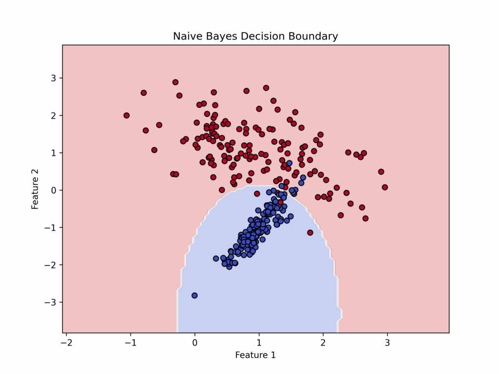
Naive Bayes also produces a “Decision Boundary” like those discussed earlier, though it differs by typically being non-linear while remaining simpler and more regular in shape.

Medical Application

The Naive Bayes algorithm has several important applications in medicine:

diagnosis and patient classification based on symptoms, laboratory tests, and risk factors
genetic sequence analysis
medical imaging

However, since medical variables are often correlated, it’s crucial to verify that the assumption of conditionally independent variables is satisfied before implementing this algorithm.

Pajila, P., Sheena, B., Gayathri, A., Aswini, J., Nalini, M., & R, S. (2023). A Comprehensive Survey on Naive Bayes Algorithm: Advantages, Limitations and Applications. 2023 4th International Conference on Smart Electronics and Communication (ICOSEC), 1228-1234. https://doi.org/10.1109/ICOSEC58147.2023.10276274.

Mohan, P., & Paramasivam, I. (2017). A Study on Impact of Dimensionality Reduction on Naïve Bayes Classifier. Indian journal of science and technology, 10, 1-4. https://doi.org/10.17485/IJST/2017/V10I20/101599.

When to Use Naive Bayes

Naive Bayes demonstrates optimal performance when dealing with features that exhibit independence from one another. This characteristic makes it especially valuable in scenarios where datasets are limited in size and computational efficiency is paramount.

The algorithm’s ability to process data rapidly, combined with its relatively simple implementation, makes it particularly well-suited for applications where quick decision-making is essential and the assumption of feature independence holds.

Limitations of using Naive Bayes

This method demonstrates reduced effectiveness in several key scenarios: when there are strong correlations between features that violate the independence assumption, when the relationships between variables play a crucial role in determining outcomes, or when working with numerical data distributions that deviate significantly from the normal distribution pattern.

In such cases, the algorithm’s fundamental assumptions may be compromised, potentially leading to suboptimal classification results and reduced model performance.

Additionally, the method’s accuracy can be particularly impacted when dealing with complex, interconnected feature sets where the independence assumption becomes increasingly unrealistic.

Variants of Naive Bayes

While this chapter has focused on Gaussian Naive Bayes (GNB), several variants exist for specific use cases:

Bernoulli Naive Bayes (BNB): used when features follow a Bernoulli distribution (0/1, True/False)
Multinomial Naive Bayes (MNB): suited for discrete and categorical data
Complement Naive Bayes (CNB): an adaptation of MNB for unbalanced datasets
Categorical Naive Bayes (CategoricalNB): designed for non-ordinal categorical features
Hybrid Naive Bayes (HNB): handles mixed feature types (both numerical and categorical)

Naive Bayes application in Python

To implement Naive Bayes in Python, we’ll create a synthetic dataset of 200 patients with four features: age, systolic blood pressure, BMI, and glucose levels.

Our target variable will be binary: disease present (1) or absent (0).

We’ll split the data into training and test sets using an 80:20 ratio.

We’ll then train a Gaussian Naive Bayes model.

After training, we’ll evaluate the model’s performance using accuracy metrics.

Finally, we’ll visualize the decision boundary between age and blood pressure.

import numpy as np
import matplotlib.pyplot as plt
from sklearn.naive_bayes import GaussianNB
from sklearn.model_selection import train_test_split
from sklearn.metrics import accuracy_score, classification_report, ConfusionMatrixDisplay

# Generate synthetic medical dataset
np.random.seed(42)
n_samples = 200

# Features: Age, Blood Pressure, BMI, Glucose Level
age = np.random.randint(30, 80, size=n_samples)
blood_pressure = np.random.randint(100, 180, size=n_samples)
bmi = np.random.uniform(18.5, 35, size=n_samples)
glucose = np.random.randint(70, 200, size=n_samples)

# Target variable (Disease: 1 = Yes, 0 = No)
disease = ((age > 50) & (blood_pressure > 140) & (glucose > 120)) | (bmi > 30)
disease = disease.astype(int)  # Convert boolean to integer

# Combine features
X = np.column_stack((age, blood_pressure, bmi, glucose))
y = disease

# Split dataset into training (80%) and testing (20%)
X_train, X_test, y_train, y_test = train_test_split(X, y, test_size=0.2, random_state=42)

# Train Gaussian Naive Bayes classifier
model = GaussianNB()
model.fit(X_train, y_train)

# Predictions
y_pred = model.predict(X_test)

# Evaluate model
accuracy = accuracy_score(y_test, y_pred)
print(f"Model Accuracy: {accuracy:.2f}")
print("\nClassification Report:\n", classification_report(y_test, y_pred))

# Display Confusion Matrix
ConfusionMatrixDisplay.from_estimator(model, X_test, y_test, cmap='Blues')
plt.title("Confusion Matrix")
plt.show()

# Visualizing decision boundaries for first two features (Age vs Blood Pressure)
def plot_decision_boundary(X, y, model):
    x_min, x_max = X[:, 0].min() - 5, X[:, 0].max() + 5
    y_min, y_max = X[:, 1].min() - 5, X[:, 1].max() + 5
    xx, yy = np.meshgrid(np.linspace(x_min, x_max, 100), np.linspace(y_min, y_max, 100))
    
    Z = model.predict(np.c_[xx.ravel(), yy.ravel(), np.full(xx.ravel().shape, 25), np.full(xx.ravel().shape, 100)])
    Z = Z.reshape(xx.shape)
    
    plt.contourf(xx, yy, Z, alpha=0.3)
    plt.scatter(X[:, 0], X[:, 1], c=y, edgecolor='k', cmap='coolwarm')
    plt.xlabel("Age")
    plt.ylabel("Blood Pressure")
    plt.title("Decision Boundary (Naive Bayes)")
    plt.show()

plot_decision_boundary(X_test, y_test, model)

import numpy as np
import matplotlib.pyplot as plt
from sklearn.naive_bayes import GaussianNB
from sklearn.model_selection import train_test_split
from sklearn.metrics import accuracy_score, classification_report, ConfusionMatrixDisplay

# Generate synthetic medical dataset
np.random.seed(42)
n_samples = 200

# Features: Age, Blood Pressure, BMI, Glucose Level
age = np.random.randint(30, 80, size=n_samples)
blood_pressure = np.random.randint(100, 180, size=n_samples)
bmi = np.random.uniform(18.5, 35, size=n_samples)
glucose = np.random.randint(70, 200, size=n_samples)

# Target variable (Disease: 1 = Yes, 0 = No)
disease = ((age > 50) & (blood_pressure > 140) & (glucose > 120)) | (bmi > 30)
disease = disease.astype(int)  # Convert boolean to integer

# Combine features
X = np.column_stack((age, blood_pressure, bmi, glucose))
y = disease

# Split dataset into training (80%) and testing (20%)
X_train, X_test, y_train, y_test = train_test_split(X, y, test_size=0.2, random_state=42)

# Train Gaussian Naive Bayes classifier
model = GaussianNB()
model.fit(X_train, y_train)

# Predictions
y_pred = model.predict(X_test)

# Evaluate model
accuracy = accuracy_score(y_test, y_pred)
print(f"Model Accuracy: {accuracy:.2f}")
print("\nClassification Report:\n", classification_report(y_test, y_pred))

# Display Confusion Matrix
ConfusionMatrixDisplay.from_estimator(model, X_test, y_test, cmap='Blues')
plt.title("Confusion Matrix")
plt.show()

# Visualizing decision boundaries for first two features (Age vs Blood Pressure)
def plot_decision_boundary(X, y, model):
    x_min, x_max = X[:, 0].min() - 5, X[:, 0].max() + 5
    y_min, y_max = X[:, 1].min() - 5, X[:, 1].max() + 5
    xx, yy = np.meshgrid(np.linspace(x_min, x_max, 100), np.linspace(y_min, y_max, 100))
    
    Z = model.predict(np.c_[xx.ravel(), yy.ravel(), np.full(xx.ravel().shape, 25), np.full(xx.ravel().shape, 100)])
    Z = Z.reshape(xx.shape)
    
    plt.contourf(xx, yy, Z, alpha=0.3)
    plt.scatter(X[:, 0], X[:, 1], c=y, edgecolor='k', cmap='coolwarm')
    plt.xlabel("Age")
    plt.ylabel("Blood Pressure")
    plt.title("Decision Boundary (Naive Bayes)")
    plt.show()

plot_decision_boundary(X_test, y_test, model)

Conclusion

Naive Bayes is a simple and efficient algorithm that adapts well to various real-world applications, particularly in medicine. However, it works best when features are at least approximately independent of each other.