micheledpierri.com: statistics, data analysis and coding

Nexus of Statistics, Data analysis, Coding, Art and Medicine

Menu
  • Home
  • Courses
    • Python Foundation
    • Statistics
    • Data Analysis
    • Machine Learning
  • Blog
    • All Pages
    • Health Informatics
    • Programming
    • Art
  • Illustrations
  • About
  • Contact
Menu
Home / Archives for Michele Danilo Pierri / Page 6

Author: Michele Danilo Pierri

Michele D. Pierri is a cardiac surgeon and cardiovascular physiopathology researcher with a strong interest in artificial intelligence, medical data science, clinical decision support, and digital health. His work focuses on the intersection between medicine, technology, and computational methods, with the aim of translating complex biomedical concepts into clear, practical, and clinically meaningful insights.
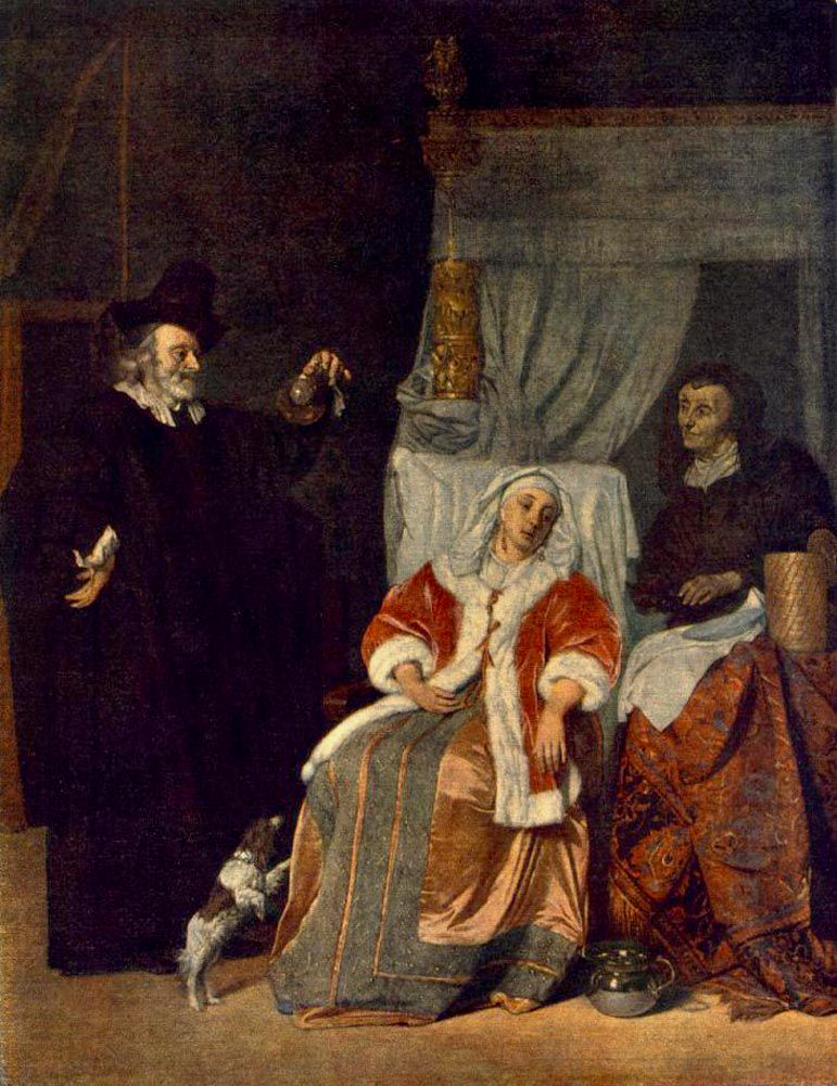
The Doctor

“The Doctor” by Luke Fildes

Posted on November 19, 2024August 11, 2026 by Michele Danilo Pierri

This highly acclaimed painting is not only a masterpiece of craftsmanship but also carries a powerful social message. It portrays the doctor as a deeply human figure, selflessly dedicated to caring for his young patient.

The Artist

Luke Fildes (1843–1927) was an English painter renowned for his portraiture. A prominent figure in Victorian art, he was keenly attuned to social dynamics—a sensitivity that permeated his artistic work. “The Doctor,” one of his most famous paintings, exemplifies this compassionate awareness.

self portrait of Sir Luke Fildes
Self-portrait of Sir Luke Fildes

The Painting

“The Doctor” depicts a physician sitting at the bedside of a sick child in a humble room.

Let’s examine the main elements of the work, focusing first on the characters:

  • The doctor, at the center of the scene, observes at the sick child. His thoughtful bearing conveys both concern and deep involvement.
  • The child lies on a makeshift bed, created by pushing chairs together, wrapped in a simple blanket. The child’s pallor and posture evoke fragility and suffering
  • In the background, the parents wait anxiously. The father observes the doctor intently, while the mother, seated near the window, buries her head in her arms—a poignant expression of worry and concern.

The environment also offers several noteworthy elements:

  • The room belongs to a poor dwelling. Sparse furniture occupies the space. A window bathes the scene in soft light, while an oil lamp suggests the nocturnal setting and the pre-electric era.

Fildes’ color palette favors dark tones, underscoring the gravity of the moment. The lighting accentuates the doctor and child, leaving the other figures in shadow.

Historical Context

The painting illustrates several typical elements of medicine during that period:

  • The doctor has no instruments—he relies solely on observation. This is his strength: the ability to observe and interpret what he sees. It reflects the diagnostic limitations of the era, when deductions were based on observation rather than technology.
  • Though severely ill, the child is cared for at home, with the doctor making a house call. This was common practice, as hospitals were reserved for the most severe cases and indigent patients.
  • The doctor’s portrayal goes beyond that of a mere technician; his entire demeanor conveys empathy and support.
  • The palpable concern of all figures surrounding the child reflects the gravity of illness in the pre-antibiotic era, when even minor ailments could prove fatal.

In the 19th century, medicine relied primarily on doctors’ observational skills and experience. The absence of instruments seen in the painting was typical for the era. Physicians like Herman Boerhaave had emphasized systematic clinical observation. During this period, René Laennec was developing the stethoscope (1816)—one of the first tools enabling more thorough patient examination.

The middle and upper classes, who could afford home care, avoided hospitals. These institutions, breeding grounds for nosocomial infections, served only the most severe cases and the poor. It wasn’t until Florence Nightingale’s work (around 1850) that hospital hygiene began to improve.

Common infectious diseases like measles, scarlet fever, and pneumonia were often fatal in the 19th century, particularly for children. Infant mortality was staggeringly high—in England, 15-20% of children died before age five.

A medical revolution was slowly unfolding. By century’s end, the landscape would change dramatically, thanks to pioneers like Louis Pasteur (germ theory), Joseph Lister (antisepsis), Alexander Fleming (penicillin discovery in 1928), and Robert Koch (bacterial infections).

Despite lacking this emerging knowledge, the doctor’s image in the 19th century evolved from the ambiguous “charlatan” of earlier times. This shift was partly due to new regulations in the medical profession. For instance, England’s General Medical Council (1858) established training standards for doctors.

Fiction, prints, and paintings also played a role in reshaping the doctor’s image—portraying them as not only competent but also humane, empathetic, altruistic, and trustworthy.

Luke Fildes’ “The Doctor,” commissioned by philanthropist Sir Henry Tate, achieved exceptional success and significantly reinforced this positive image of the medical profession.

A physician stands on a glowing divide between two opposing worlds: a dark quarantined industrial city with masked medical staff on one side, and a fiery militarized landscape with rows of soldiers and an authoritarian flag on the other.

Dr Rieux in Albert Camus’ “The Plague”

Posted on November 10, 2024August 11, 2026 by Michele Danilo Pierri

The Author

Albert Camus (1913–1960) was a French writer-philosopher and a key figure in existentialism.

Born in Mondovi, Algeria, Camus began his philosophy studies in Algiers. He later moved to Paris where, during World War II, he actively participated in the resistance against Nazi occupation. His most renowned novel is “The Stranger.” In 1957, Camus was awarded the Nobel Prize in Literature.

Albert Camus' photo

“The Plague”

The novel is set in the Algerian city of Oran and chronicles a sudden plague epidemic that ravages the city.

Dr. Rieux serves as both narrator and protagonist, presenting the story as a firsthand account of the events.

Dr. Rieux, too, stood up. He was of medium height, broad-shouldered, and square-set. The brisk and energetic movements of his head, with its dark, steady eyes and firm mouth, suggested a man who was tenacious in purpose. His manner was direct, and he had a certain geniality of expression which never forsook him, even in his moments of irritability.

The narrative begins with the ominous discovery of dead rats—a warning sign overlooked by both authorities and citizens.

But what had happened in the last few days was quite out of the ordinary and, to his thinking, disquieting. For one thing, it was a fact that in this metropolis rodents were quite out of place, yet here they were, each day bringing in its train several hundred fresh rats, swept out of cellars and attics, to die in the open.”

Only when patients exhibiting high fever, swollen lymph nodes, and sudden deaths emerge does the diagnosis of bubonic plague send the population into panic.

Authorities place the city under strict quarantine, isolating it from the outside world. This isolation prevents communication even between family members, creating an extremely traumatic experience for the populace.

Rieux was astonished to find how easy it was to stop thinking clearly, how easy it was to lapse into a dream-like state where things happened of their own accord. In this state men could think of nothing but ‘the plague.’ All day they were caught up in an unbroken stream of rumors and alarms, one succeeding another.

As the infection spreads, the population’s reactions vary widely, ranging from apathy to moments of profound solidarity.

After several months, the epidemic begins to wane. Many have perished, and the survivors are deeply scarred by the experience. Dr. Rieux reflects that this event serves as a stark reminder of humanity’s enduring vulnerability.

Oran city, Algery in 1943
Oran city, Algery actually

The Novel from a Medical History Perspective

The novel transports us to the world in the middle of 20th-century medicine, depicting both its capacity to respond to disease outbreaks and the public’s perception of medical practices during that era.

Key aspects of the novel from a medical history perspective:

  • Response to the epidemic: Initially underestimated, authorities soon impose strict isolation and quarantine measures. This mirrors historical responses to epidemics, as limited therapeutic and preventive capabilities made these the primary public health measures available.
  • Therapeutic capacity: Dr. Rieux’s treatments are largely palliative and ineffective, reflecting medicine’s powerlessness against such infectious diseases before the advent of antibiotics and vaccines.
  • Medical ethics: Dr. Rieux embodies a new portrayal of doctors, contrasting with previous centuries. Rather than a self-interested figure exploiting popular credulity and serving only the elite, he’s a people’s doctor who disregards social status and offers his limited abilities to all patients equally.

His profession required him to keep away from abstractions. ‘Only one idea was clear in his mind: that he was here to attend to the sick. And he had resolved to do that without a moment’s deflection. That, too, was a beginning. But it was no more than a beginning.

For who would dare to assert that eternal happiness can compensate for a single moment’s human suffering? Rieux had heard a mother crying for her dead child, and that cry remained with him… His job was to attend to them, to put his professionalism at the service of those who suffered, without questioning whether it was worth it or not.

Rieux said he knew the plague had cost him the power of emotion, and even the faculty of loving someone. Only love and duty made men endure their pain.

The work also reveals that disease, particularly the plague, was often perceived as divine retribution for collective sins. This view persisted for a long time, despite medical advancements.

Rieux knew now that the plague was here and that he must do his best to fight it. He remembered a phrase of his friend Tarrou: ‘Each of us has the plague within him; no one, no one on earth is free from it. And I know, too, that we must keep endless watch on ourselves lest in a careless moment we breathe in somebody’s face and fasten the infection on him.

Furthermore, it highlights a growing sense of solidarity among the afflicted populations and demonstrates how the epidemic catalyzed efforts to strengthen and better organize healthcare structures.

Dr. Rieux resolved to keep silent and stay in the fight… He knew that the tale he had to tell could not be one of final victory. It could only be the record of what had to be done, and what, no doubt, would have to be done again in the never-ending fight against terror and its relentless onslaught.

This work holds significant importance from a medical history perspective. It serves as a powerful reminder of society’s vulnerability to epidemics, even in the face of advancing medical knowledge. The novel emphasizes the critical necessity for unwavering medical ethics, particularly during times of crisis when ethical boundaries may be tested. It vividly highlights the paramount importance of strengthening control and prevention measures in public health systems, demonstrating how these can make a substantial difference in managing outbreaks. Furthermore, the narrative underscores the invaluable lessons that can be extracted from past events, emphasizing how this historical knowledge can be utilized to better prepare for and respond to inevitable future outbreaks.


Nazists in Paris
Attribution: Bundesarchiv, Bild 183-H28708 / Heinrich Hoffmann / CC-BY-SA 3.0

There is, however, a second layer of interpretation that uses medicine as a metaphor for France’s political situation during the Nazi occupation.

This reading highlights how the “disease,” with its ever-present destructive force, can be seen as a metaphor for the Nazism oppressing France at that time.

Dr. Rieux, in this context, becomes a symbol of resistance against this metaphorical plague. He confronts it as he does the literal plague in the novel: organizing responses, aiding the suffering, and persevering in his actions—even while aware of his limited power to combat the “infection.”

The quarantine and isolation of Oran can be interpreted as a reference to the invasive and oppressive control the occupiers imposed on the population.

Lastly, the initial underestimation that allowed the contagion to spread, followed by the resolve to learn from these events, mirrors the determination to be better prepared when the metaphorical bacillus—which can never be fully defeated—inevitably returns.

Through its compelling storytelling, “The Plague” not only entertains but also educates, leaving readers with a deeper understanding of the complex interplay between medicine, society, and human nature during times of widespread illness.

Images from Wikimedia Commons

A physician in a white coat examines the arm of a young woman resting in an iron hospital bed, surrounded by antique medical instruments in a warmly lit early 20th-century ward.

Doctor Grenvil in Giuseppe Verdi’s La Traviata

Posted on October 30, 2024August 5, 2026 by Michele Danilo Pierri

Scene: Violetta’s room. It is morning; the room is elegantly furnished but shows signs of her illness and poverty. Violetta is lying in bed, visibly weak. Annina is close to her. Dr. Grenvil enters.

Annina: How is she, doctor?

Dr. Grenvil: Alas, she is very ill. She has little time left… it’s agony. Consumption has finally conquered her.

Annina:What sorrow! What fate!

Giuseppe Verdi's portrait

The story

“La Traviata,” an opera composed by Giuseppe Verdi, tells the love story of Violetta Valéry and Alfredo Germont. Their happiness is cut short when Violetta is asked by Alfredo’s father to leave him. Alfredo initially believes this to be a betrayal. However, after learning the reason for their separation, he rushes to Violetta’s side. He finds her gravely ill with tuberculosis, and she dies in his arms.

Doctor Grenvil

Doctor Grenvil, though a minor character in the opera, plays a crucial role in its structure. He visits Violetta and, upon assessing her health, informs Annina, Violetta’s maid, of her condition.

In the final ensemble, Grenvil expresses his powerlessness against Violetta’s illness and joins the other characters in their despair.

Despite his limited role, Doctor Grenvil serves as an important element of moderation, presenting a rational and empathetic presence amidst the opera’s passionate and tragic context.

He is one of the few characters to show genuine concern for Violetta’s well-being. His role extends beyond merely informing the characters—and by extension, the audience—of the protagonist’s terminal condition; he highlights Violetta’s vulnerability and isolation. Grenvil treats her with attention and respect when others condemn her. With his authority and rationality, he remains above the tumultuous emotions while still embodying a deeply human figure.

The Medical Context of the Era

Set in the 19th century, Violetta’s story was tragically common. Tuberculosis, then known as “consumption,” was rampant throughout Europe. Doctors were powerless against the disease, with no specific treatments available. They could only suggest palliatives such as rest and, when possible, living in healthier environments.

Despite his inability to cure, Dr. Grenvil demonstrates empathy, continuing to care for Violetta and remaining by her side. This aligns with the medical ethics of the era—even when scientifically helpless, doctors maintained their commitment to patient care. This “solidarity” is poignantly illustrated in the story’s final moments, as the dying Violetta finds comfort in Dr. Grenvil’s supportive presence.

Grenvil embodies the 19th-century vision of a doctor prevalent in artistic and literary works—a figure both rationally detached and deeply empathetic. He represents a pivotal moment in medical history, as the profession began to shed superstitious practices and establish itself as a science.

Similar portrayals of doctors appear in other literary works: Dr. Manette in Dickens’s “A Tale of Two Cities,” the rational and empathetic Dr. Watson in Arthur Conan Doyle’s “Sherlock Holmes” series, and Dr. Rieux in Camus’s “The Plague”—a doctor who, like Grenvil, battles against an inexorable fate in the late 19th century.

Images from Wikimedia Commons

A masked technician in an early 20th-century laboratory examines a long strip of medical film beside a large mechanical projector, surrounded by analog control panels, surgical instruments, and a glowing circular image on the wall.

Inside Dicom

Posted on October 29, 2024August 11, 2026 by Michele Danilo Pierri

In a previous blog post, we explored how to read the content of a DICOM file, including its numerous tags. These tags provide insights into the study type, characteristics, and all relevant patient and study information.

Now, we’ll focus on the most crucial tag—the one containing the images. A typical study can include anywhere from a few to several hundred DICOM files, usually identifiable by their .dcm extension.

For our practice, we’ll open a single .dcm file containing a frontal projection chest X-ray.

Environment Setup

Before we begin, it’s essential to install some key libraries. Due to dependency issues, it’s best to create a dedicated environment for running Python with these libraries. In our environment, we’ve installed numpy, pandas, and matplotlib—common libraries for data management and visualization—as well as the pydicom library discussed in our previous post.

For this specific task, we’ve also installed these additional libraries:

scipy: An open-source library for scientific computing in Python, based on numpy. It’s particularly useful for applying image transformation filters.

opencv (cv2): The Open Source Computer Vision Library, which uses machine learning for computer vision tasks. It provides various tools for image processing. In Python, you can access it through the cv2 module.

pylibjpeg, pylibjpeg-libjpeg, and gdcm: These libraries are necessary for working with and processing DICOM files.

Our radiographic image is located at IMAGES\01\00001.dcm on a diagnostic CD. It contains a frontal projection chest X-ray. The same directory also includes file 00002.dcm, which contains the lateral projection—we won’t be using this for now.

Loading the image

First, let’s import the necessary libraries:

import pydicom
import matplotlib.pyplot as plt
import numpy as np

Now, we’ll locate our .dcm file and load the dataset into the dicom_data variable.

The image data in dicom_data is stored in the pixel_array attribute, which we’ll assign to the image variable. This creates a numpy array of rows and columns containing the pixel data that forms the image.

# Specify the path to the DICOM file
dicom_path = "C:\\Dicom\\RX\\IMAGES\\01\\00001"

# Read the DICOM file
dicom_data = pydicom.dcmread(dicom_path)

# Extract the image from the DICOM dataset
image = dicom_data.pixel_array:

Let’s extract some key information about our image: its data type, dimensions in pixels, and the range of possible pixel values:

# Information about the array
print("Pixel data type:", image.dtype)
print("Image dimensions:", image.shape)
print("Maximum pixel value:", np.max(image))
print("Minimum pixel value:", np.min(image))

Pixel data type: uint16 Image

dimensions: (2400, 2880)

Maximum pixel value: 4095

Minimum pixel value: 0

Our image has dimensions of 2400 x 2880 pixels, with each pixel capable of holding a value from 0 to 4095.

The pixel data type indicates a bit depth of 16 unsigned bits (u) per pixel, allowing for 2^16 = 65,536 grayscale values (opacity and brightness) ranging from 0 to 65,535. In contrast, an 8-bit image has a lower depth, with each value on the scale ranging from 0 to 255 (2^8 = 256 values).

However, it’s worth noting that while the data type allows for up to 65,535 values, the actual image in this case only uses values from 0 to 4095. This suggests that the image is effectively using 12 bits of information (2^12 = 4096 possible values), even though it’s stored in a 16-bit format.

Medical images are typically stored in 12- or 16-bit formats. The lowest values (0) correspond to darker areas in the image.

We can visualize the image using matplotlib:

# Display the image
plt.imshow(image, cmap="gray")
plt.axis("off")  # Hide axes for a clean visualization
plt.show()

The resulting image will be displayed as follows:

chest X-ray

Out of curiosity, let’s extract the values from a small 10×10 pixel area of the image, read the stored values, and reconstruct them based on the grayscale.

# Define the starting position for the square (you can modify it based on your needs)
start_x, start_y = 100, 100  # For example, the top-left pixel of the square

# Extract a 10x10 pixel square from the resized frontal image
square = image[start_y:start_y+10, start_x:start_x+10]

# Display the numerical values of the pixels
fig, axes = plt.subplots(1, 2, figsize=(12, 6))

# First grid: numerical pixel values
axes[0].imshow(square, cmap="gray")
for i in range(10):
    for j in range(10):
        # Insert the pixel value at the center of the cell
        axes[0].text(j, i, int(square[i, j]), ha="center", va="center", color="red", fontsize=10)
axes[0].set_title("Pixel Values")
axes[0].axis("off")  # Remove axes for a clean visualization

# Second grid: grayscale
axes[1].imshow(square, cmap="gray")
axes[1].set_title("Grayscale")
axes[1].axis("off")

# Optimize the layout
plt.tight_layout()
plt.show()

pixels

Various operations can be performed on the pixel matrix that composes the image. Let’s explore a few of them.

Normalization

When the grayscale range is extensive (in our case, from 0 to 65,535), it’s often beneficial to normalize it to a scale of 0 to 255. This process can enhance the visibility of details perchè con valori di intensità molto distanti potrebbero essere non distinguibili.

When the grayscale range is extensive (in our case, from 0 to 65,535), it’s often beneficial to normalize it to a scale of 0 to 255. This process can enhance the visibility of details, as intensity values that are very far apart might otherwise be indistinguishable to the human eye.

# Normalization between 0 and 255
image_normalized = (image - np.min(image)) / (np.max(image) - np.min(image)) * 255
image_normalized = image_normalized.astype(np.uint8)

# Display the normalized image
plt.imshow(image_normalized, cmap="gray")
plt.title("Normalized Image")
plt.axis("off")
plt.show()

chest X-ray  after normalization

Equalization

This technique adjusts pixel values to better distribute intensities across the image. It’s particularly useful for radiographic images as it enhances the visibility of structures that are otherwise difficult to perceive.

To perform equalization, we’ll use the cv2 library:

import cv2

# Histogram equalization with OpenCV
image_equalized = cv2.equalizeHist(image_normalized)
plt.imshow(image_equalized, cmap="gray")
plt.title("Image with Histogram Equalization")
plt.axis("off")
plt.show()

chest X-ray after equalization

Smoothing or Gaussian Filter

The Gaussian filter averages nearby pixels to reduce sudden value variations and noise. As a result, images appear less detailed but more uniform.

You can import the Gaussian filter from scipy.

from scipy.ndimage import gaussian_filter

# Apply a Gaussian filter to reduce noise
image_smoothed = gaussian_filter(image_normalized, sigma=1)

# Display the image with smoothing
plt.imshow(image_smoothed, cmap="gray")
plt.title("Image with Smoothing (Gaussian Filter)")
plt.axis("off")
plt.show()

chest X-ray following application of smoothing

Pseudocoloring

Pseudocoloring applies filters to colorize areas in grayscale images, enhancing visual analysis. For instance, the “jet” filter assigns blue to low intensities and red to high intensities, making different regions more distinguishable.

# Apply a "jet" color map for pseudo-coloring
plt.imshow(image_normalized, cmap="jet")
plt.title("Pseudo-Colored Image")
plt.axis("off")
plt.colorbar()  # Add a color bar for reference
plt.show()

chest X-ray pseudocolored

Another color scale option is the cool/warm scale:

plt.imshow(image_normalized, cmap="coolwarm")
plt.title("Image with Cool/Warm Coloration")
plt.axis("off")
plt.colorbar()
plt.show()

chest X-ray with cool-warm coloration

Thresholding

The image is converted to binary, with pixels below a certain threshold becoming black and those above turning white. This process highlights high-density elements like bones in an X-ray.

threshold_value = 128  # Example threshold, to be adapted to the image
image_thresholded = (image_normalized > threshold_value) * 255

plt.imshow(image_thresholded, cmap="gray")
plt.title("Image with Intensity Threshold")
plt.axis("off")
plt.show()

chest X-ray with intensity threshold

Edge Detection (Canny)

The Canny edge detection algorithm identifies edges in an image based on intensity gradients. It uses two threshold values to determine which edges to keep.

# Apply edge detection using OpenCV's Canny method
edges = cv2.Canny(image_normalized, threshold1=30, threshold2=34)

# Display the detected edges
plt.imshow(edges, cmap="gray")
plt.title("Image with Edge Detection (Canny)")
plt.axis("off")
plt.show()

chest X-ray after application of edge detection

Thresholding and edge detection share a limitation: they separate structures on the basis of pixel intensity alone, with no notion of what the structure actually is. A bone edge and a catheter edge look the same to Canny. Identifying which pixels belong to a given anatomical structure requires semantic segmentation, and the reference architecture for medical images is UNet, designed precisely to work with the small annotated datasets that clinical research typically produces.


With the pixel matrix that composes an image at our disposal, we have a wide array of manipulation techniques to enhance its visualization. These techniques allow us to extract more information, highlight specific features, or improve the overall clarity of the image.

In many medical imaging scenarios, we often encounter multiple images of the same patient and anatomical region. This presents exciting opportunities beyond single-image manipulation. We can use these multiple images to reconstruct three-dimensional volumes, providing a more comprehensive view of the anatomy. Additionally, we can create dynamic sequences or moving images, which can be particularly useful for studying physiological processes or changes over time.

These advanced processing techniques, such as volume reconstruction and dynamic imaging, open up new possibilities for diagnosis, treatment planning, and medical research. They allow healthcare professionals to gain deeper insights into patient anatomy and physiology, potentially leading to more accurate diagnoses and improved patient care

An elderly bearded scholar sits among open books in the ruins of a devastated city, speaking to a young boy as a crumbling cathedral rises in the background.

“The Scarlet Plague” by Jack London

Posted on October 26, 2024August 5, 2026 by Michele Danilo Pierri

I alone remember. And if I don’t tell you, children, everything that was and everything we knew, all will be lost.


Jack London (1867–1916) was a prolific American writer. He’s best known for adventure novels like “The Call of the Wild” and “White Fang,” but his vast work also addressed social issues.

Jack London's photo

“The Scarlet Plague,” a short novel written in 1912, is notable for being one of the first post-apocalyptic novels in modern literature.

The historical references that likely inspired the author were the plague and cholera epidemics (as depicted in the stories of Boccaccio and Defoe). These occurred during periods when medicine was still in its infancy and lacked effective remedies against diseases. Interestingly, the Spanish flu pandemic itself emerged after London had written this story (1918–19).


The Story

Set in 2073, exactly 70 years after a catastrophic epidemic—the scarlet plague—decimated humanity, the story depicts a world where survivors have regressed to a primitive state.

Professor James Howard Smith narrates the events leading to this outcome, aiming to pass on the memory of the plague and its consequences to future generations.

The scarlet plague, whose clinical and epidemiological characteristics the author doesn’t elaborate on, was marked by an extremely high transmission rate and mortality. Its severe virulence and the inability to mount an effective response led to widespread panic and chaos.

It was a frightful epidemic. People were dying like flies. The disease killed within minutes and the infection spread like wildfire. People were seized by desperate panic, and everything descended into chaos.

Cities crumble, infrastructure collapses, and the few survivors gather in small, isolated communities. They revert to a state of barbarism where civil achievements and medical knowledge fade into obscurity. Centuries of scientific discoveries vanish, lost to time.

Everything has been lost. Not just civilization, but everything that was part of it. Science, medicine, all knowledge… nothing remains anymore

Healthcare systems were the first to collapse, unable to respond to the pandemic and lacking the resilience to survive it. Hospitals became viewed more as sources of contagion than places of treatment.

The cities emptied out. Hospitals were abandoned, no one had the courage to approach the sick. The government dissolved and people sought refuge in nature, far from the contagion

Doctors, in particular, were astounded by the speed and lethality of the unknown disease. Unable to identify its cause, they tragically became victims themselves.

“Doctors were brave, some of them died while trying to treat others, but nothing could stop the scarlet plague. There was no cure, there was no hope.

The post-pandemic state of barbarism, along with the loss of medical knowledge and basic health norms, demonstrates the fragility of scientific achievements and hygiene practices we often take for granted. This stark reality underscores the critical importance of careful public health management.

Without the knowledge of the past, men have returned to barbarism, no longer caring about hygiene or medicine. We live like beasts, devoid of the most basic standards of cleanliness


Ancient and Modern Pandemics

Jack London’s “The Scarlet Plague” demonstrates a remarkable foresight that echoes with our recent experience of the Covid-19 pandemic.

bacteria

While the coronavirus certainly exhibited less virulence than London’s fictional “scarlet plague,” the parallels between the imagined events and our lived reality in 2020 are both striking and thought-provoking.

London’s prescient narrative serves as a reminder of how literature can sometimes anticipate future challenges, offering valuable insights into human behavior and societal responses during times of crisis.

The Covid-19 pandemic, although less severe, bears numerous similarities to London’s fictional “scarlet plague,” especially in its early stages.

The novel coronavirus vividly illustrated the rapidity with which pathogens can proliferate on a global scale in our interconnected world.

London’s work anticipated with accuracy the immense strain placed on healthcare systems worldwide. We witnessed overwhelmed hospitals, critical shortages of essential medical equipment such as ventilators, and healthcare professionals working under unprecedented pressure and personal risk.

street washing during the covid pandemic

In the period before the development and distribution of vaccines, society grappled with a pervasive uncertainty about how to effectively control the pandemic’s spread. This uncertainty led to the implementation of extreme measures, including widespread lockdowns, which echoed the drastic actions taken in London’s narrative.

Many individuals experienced a degree of isolation and fear reminiscent of London’s characters, albeit to a lesser extent.

deserted streets during the lockdown

I wasn’t scared. I had been exposed to the contagion and already considered myself dead. What struck me wasn’t this, but a feeling of tremendous depression. Everything had stopped. It seemed like the end of the world, of my world.

The pandemic brought to the forefront both the best and worst aspects of human nature, revealing a complex interplay of solidarity and self-interest.

Yet, even in despair, men were men. We fought, loved, cried, as we did before. The plague could not take away who we were.

While our society did not descend into the barbarism depicted in “The Scarlet Plague” – thanks in large part to successful epidemic control measures and scientific advancements – the crisis nonetheless exposed vulnerabilities in our social fabric and tested the resilience of our institutions.

Messages

The work imparts several messages that remain profoundly relevant in our current times:

  • We cannot predict the emergence of new pathogens responsible for epidemic diseases, which can spread rapidly. Therefore, health organizations must be prepared to manage unforeseen situations with adequate reserves of personnel, equipment, and knowledge. Efficient healthcare systems are crucial not only for combating diseases but also for maintaining social cohesion by supporting populations during crises.
  • It is vital to preserve, share, and document medical progress. Training, dissemination, and global access to medical knowledge must be guaranteed even in the face of catastrophic events. The loss of such knowledge would make any disaster even more devastating.
  • Panic and disorganization during catastrophic and unforeseen events must be avoided. The healthcare sector, as well as other social organizations, must be prepared—both logistically and psychologically—to face these challenges.

Civilization is a thin veil. And without it, we have returned to what we once were, before we learned to govern ourselves, before we invented laws and moral principles.

Images from Wikimedia Commons

A wide, painterly vintage seascape shows a solitary scholar standing on a rocky cliff beside books and a globe, looking out over three small islands in the sea. The islands are clearly separated, while the waters around them vary from calm and circular to rough and turbulent, creating a poetic visual metaphor for comparison and variation.

F statistic

Posted on October 21, 2024June 20, 2026 by Michele Danilo Pierri

Both one-way ANOVA (Analysis of Variance) and repeated measures ANOVA employ the F statistic as a tool to evaluate the null hypothesis that there are no significant differences between the groups being studied.

Numerous other statistical tests utilize the F statistic, including regression, Levene’s and Bartlett’s tests for homogeneity of variance, MANOVA, ANCOVA, Wilks’ lambda test, and Mauchly’s test of sphericity.

The F statistic operates by conducting a comparative analysis of two estimated variances.

The first of these is the between-group variance, which is indicative of systematic differences that may exist across the groups. This variance captures the extent to which the groups differ from one another in a consistent, non-random manner.

The second variance examined is the within-groups variance, representing the random variability present within each group.

The more the between-group variability exceeds the within-group variability, the higher the F value becomes, indicating a greater likelihood that the groups are significantly different.

How is the F statistic calculated? Let’s explore this using simple examples with small numbers to illustrate how the F statistic is derived.

Let’s consider a scenario where we compare three groups of three patients each, subjected to different treatments (A, B, and C). The treatment results are as follows:

GroupResults
A5, 6, 7
B8, 9, 7
C10, 10, 11

We can easily calculate the means of groups A, B, and C, as well as the overall mean:

\mu_A=\frac{5+6+7}{3}=6

\mu_B=\frac{8+9+7}{3}=8

\mu_C=\frac{10+10+11}{3}=10.33

*** QuickLaTeX cannot compile formula:
\mu_T_O_T=\frac{5+6+7+8+9+7+10+10+11}{9}=8.22

*** Error message:
Double subscript.
leading text: $\mu_T_

The sum of squares between groups (SSB) quantifies the extent to which group means deviate from the overall mean.

SSB = n_A(\mu_A-\mu_{TOT})^2 + n_B(\mu_B-\mu_{TOT})^2 + n_C(\mu_C-\mu_{TOT})^2

SSB = 3(6-8.22)^2 + 3(8-8.22)^2 + 3(10.33-8.22)^2

SSB = 28.212

The sum of squares within groups (SSW) is calculated as follows:

SSW = \sum_{i=1}^{n_A}(x_{iA}-\mu_A)^2 + \sum_{i=1}^{n_B}(x_{iB}-\mu_B)^2 + \sum_{i=1}^{n_C}(x_{iC}-\mu_C)^2

Group A = (5−6)^2 + (6−6)^2 + (7−6)^2 = 2

Group B = (8−8)^2 + (9−8)^2 + (7−8)^2 = 2

Group C = (10−10.33)^2 + (10−10.33)^2 + (11−10.33)^2 = 0.67

SSW = 4.67

Let’s proceed with calculating the degrees of freedom (df):

Between groups = df_B = 3-1 = 2

Within groups =df_W = 9-3 = 6

Finally, we calculate the Mean Squares for Between Groups (MSB) and Within (MSW) Groups:

MSB = SSB/df_B = 28.212/2 = 14.106

MSW = SSW/df_W = 4.67/6 = 0.778

The F statistic is the ratio of MSB to MSW, thus

F = MSB/MSW = 14.106/0.778 = 18.13

In repeated measures ANOVA, the calculations follow a similar pattern to one-way ANOVA, but there’s a crucial difference in how the concept of “group” is applied. Instead of comparing different groups of subjects, repeated measures ANOVA focuses on the individual subject as the unit of analysis. In this context, each subject essentially becomes their own “group,” with the repeated measurements taken from that subject over time or under different conditions forming the data points within that group.

For instance, if we’re studying the effects of a new medication on blood pressure, we might measure each participant’s blood pressure at baseline, after one week of treatment, and after one month of treatment. In this case, each participant’s set of three measurements would constitute a “group” in the repeated measures ANOVA framework.

Early 20th-century doctor in a white coat examines a seated woman wrapped in a blanket inside a modest rural clinic, with wooden furniture, medicine bottles, an oil lamp, and snow-covered windows.

“A Young Doctor’s Notebook” by Mikhail Bulgakov

Posted on October 17, 2024August 9, 2026 by Michele Danilo Pierri

“A Young Doctor’s Notebook” by Mikhail Bulgakov is a goldmine of information for those interested in the history of medicine.

Mikhail Bulgakov, a Russian doctor and writer, lived from 1891 to 1940. Born into a family of intellectuals, he studied medicine in Kiev, graduating in 1916. He then worked in various rural villages, with his first experience in Smolensk, Russia, proving particularly formative. Many events narrated in “A Young Doctor’s Notebook” stem from this experience.

After contracting typhus during his medical work, Bulgakov gradually abandoned the profession to dedicate himself to writing. Among his notable works is “The Master and Margarita,” widely regarded as his masterpiece. He died in Moscow in 1940 and is now considered one of the greatest Russian writers.

Mikhail Bulgakov's photo

In “A Young Doctor’s Notebook,” Bulgakov recounts the experiences of a young physician sent to a remote village in rural Russia shortly after the 1917 revolution. The work offers numerous accounts of the state of medicine in rural Russia during this period of profound social transformation.


The young, inexperienced doctor finds himself isolated. He has no nearby medical facilities for referrals, no seasoned colleagues to seek advice from and no possibility of specialist consultations.

This isolation, characteristic of rural doctors, subjected the young physician to constant pressure and challenges. He faced a lack of support and feared confronting difficult situations without the necessary experience.

“I found myself completely alone, a newly graduated doctor, with only four years of theory behind me, thrown into a hole, without the possibility of receiving advice from anyone.”

Lack of resources

The medical facilities lacked adequate diagnostic tools, even those limited ones available at the time. Medicines were scarce, a situation exacerbated by the post-revolutionary period’s disorganization. This situation led to a profound sense of frustration in the young doctor.

For instance, when faced with performing an emergency tracheotomy, he discovers he lacks the proper tools:

“I lacked the necessary instruments. I didn’t have a complete tracheotomy set. The knife I found was barely suitable and I felt like a butcher.”

Theoretical Knowledge vs. Practical Experience

The transition from theoretical knowledge gained in university to the demanding realities of clinical practice is a common challenge for doctors across different eras and locations. This gap between theory and practice often creates a sense of inadequacy. For the protagonist, this feeling is particularly acute due to his isolation and lack of resources—conditions that intensify the struggle faced by many young physicians.

A striking example occurs when the young doctor faces the daunting task of performing an amputation:

“There was a mountain of muscles, arteries, veins, and everything was moving. The textbook hadn’t prepared me for this. Muscles had never been part of my exam.”

Hygienic and Sanitary Conditions

The protagonist encounters deplorable hygienic and sanitary conditions among the rural population. Infectious diseases run rampant, and patients lack awareness of even the most basic hygiene practices.

“The woman presented herself with mud-caked feet, a filthy scarf on her head, and obvious signs of syphilis. She had no idea what hygiene was. She had never seen a doctor before.”

Medical Progress

Despite adverse conditions and limited resources, the young doctor recognizes significant advancements in his field. He consistently strives to maintain a scientific approach in his practice. When successfully employing a remarkable new technique during a challenging childbirth, he experiences joy and appreciation for the progress he witnesses firsthand.

“Thanks to chloroform, the operation was successful. It was the first time I had used an anesthetic, and it seemed incredible to be able to operate without causing pain.”

picture of town with snow

The pathologies encountered by the young doctor offer insight into the diseases prevalent in rural areas during the early 20th century.

Syphilis

Syphilis was one of the most common conditions treated by the young doctor. This sexually transmitted disease was rampant among the poorest social classes. It manifested through skin lesions (ulcers or eruptions) and systemic symptoms. Patients often sought medical attention only at an advanced stage. Since antibiotics hadn’t been invented yet, treatment relied on mercury or Salvarsan—a chemotherapeutic drug introduced in 1910.

“Every patient with signs of syphilis was terrified by the word ‘Salvarsan,’ refused to follow my prescriptions, and preferred to rely on folk medicine remedies.”

Diphtheria

Diphtheria was even more feared than syphilis, primarily because it affected children. High fever and breathing difficulties raised suspicions of the disease, with diagnosis confirmed by the presence of grayish membranes in the throat.

Though antitoxin serums had been introduced by this time, they were rarely available in rural areas. The only life-saving remedy, therefore, remained emergency tracheotomy.

“I’d never performed a tracheotomy before, but I had no choice. The child was suffocating.”

Typhus

Typhus was another prevalent infectious disease in rural populations, exacerbated by poor hygiene. It presented with fever, abdominal pain, and diarrhea, accompanied by a distinctive rash. Before the advent of antibiotics, no effective cure existed. Doctors could only offer supportive care, focusing on hydration and fever management.

“The hygienic conditions in the village were terrible, and each winter brought new waves of typhus.”

Complicated Childbirth

In that era, doctors could only identify a complicated childbirth through prolonged labor and the fetus’s abnormal position. Modern monitoring systems were nonexistent. Manual techniques proved largely ineffective, often necessitating the use of forceps to perform an assisted delivery. Inoltre non c’era l’anestesia e quindi questi interventi erano molto dolorosi. Additionally, the absence of anesthesia meant these procedures were excruciatingly painful.

“My hands were trembling as I tried to apply the forceps. It felt like I was holding not just a baby, but life itself in my hands, and I could only pray that everything would go well.”

Wounds and Injuries

Farm work frequently led to wounds or injuries, which occasionally resulted from violent incidents as well. The doctor’s treatment involved suturing, placing drains, and cleansing with antiseptics—primarily iodine and alcohol—to ward off infections.

“I had no means to prevent infection. I could only clean the wound as best as possible and hope it wouldn’t worsen.”


A central aspect of Bulgakov’s narrative is the contrast between theoretical training and practical reality, particularly in the rural and ill-equipped setting where he began his medical career.

The young doctor immediately perceives the stark contrast between his theoretical training and the practical realities of rural medicine, causing him considerable anxiety:

“I had studied the manuals, I had passed the exams, but nothing had prepared me for what I found here. The human body didn’t seem to be the same as described in my textbooks.”

This contrast between theory and practice breeds a sense of inadequacy, manifesting as intense anxiety and fear when confronting complex emergencies. Furthermore, the weight of responsibility is immense, as the doctor realizes that a patient’s life hangs in the balance of their every decision and action.

“My hands were trembling. I had never seen anything like it, let alone done it. But I couldn’t back down. The patient’s life was in my hands.”

Finally, there’s the realization that beyond the gap between theory and practice lies a reality surpassing what was taught. The young doctor encounters situations never addressed during his studies, forcing him to confront unforeseen challenges.

“The book said everything would go smoothly, but reality bore no resemblance to anything I had studied. The childbirth wasn’t proceeding as expected, and I felt lost.”

Despite this abyss of inadequacy, anxiety, and terror, the doctor summons the strength to resolve situations—inventing, adapting, and improvising.

“There was no time for doubt. I had to act. I took the scalpel and made the incision. I had never done it before, but I had no choice.”

Through facing novel and unforeseen situations, the doctor gradually builds confidence and skills. Learning on the job—with both successes and failures—he gains practical competence that his studies hadn’t provided. This hands-on experience, filled with trials and errors, proves invaluable in developing abilities beyond what textbooks could offer.

“After each procedure, I felt a new awareness growing within me. Every mistake, every success taught me something that no book had ever taught me.”


A final aspect worth exploring in Bulgakov’s text is the doctor’s relationship with patients and the broader community. The villagers’ shifting attitudes, their expectations, and their tendency to glorify successes while assigning blame for failures remain surprisingly relevant today. This dynamic between medical professionals and the public they serve continues to be a complex and often challenging aspect of healthcare.

Initially, when the young doctor arrives in the village, he is viewed with admiration. The villagers see him as an authoritative figure capable of curing diseases and solving problems. To them, he represents not only a bearer of scientific and modern knowledge but also a sort of possessor of esoteric powers.

“They looked at me and my bag with a sort of veneration. I was the first doctor they had ever seen in the flesh, and to them, I was a magical figure.”

However, as treatments fail to yield immediate results and his prescriptions stray from popular beliefs, the villagers’ initial admiration swiftly morphs into distrust and suspicion.

“Despite my best intentions, they continued to believe that their folk remedies were more effective than my medicines. They often looked at me with suspicion, as if they didn’t really trust what I was doing.”

Beyond the aspects we’ve already discussed, the doctor faces an additional source of anxiety: the knowledge that a single mistake or failure could irreparably damage his reputation. For instance, following a challenging delivery resulting in the infant’s death, the community’s regard for the doctor drop dramatically.

“After the baby’s death, I felt they looked at me differently. I was no longer the promising young doctor who would solve every problem. Now I was simply another fallible man.”

The villagers clung to their folk remedies and superstitions, often viewing the doctor’s modern treatments with suspicion and fear. This realization led the young physician to understand that his role extended beyond merely treating patients—he needed to educate them as well.

“When I prescribed a medication, they often refused it, preferring to rely on a spell or an ointment passed down from their ancestors.”

However, trust and confidence can be as quickly regained as they were lost, following a successful intervention and a patient’s recovery.

“After the operation, they looked at me as if I were a living miracle. I had brought someone back to life whom they had already given up for dead. For the first time, I felt the weight of my power.”

The relationship between doctors and patients in Russian rural villages continues to be characterized by a complex and ever-shifting dynamic in the modern era. This fluctuation in sentiment ranges from eager anticipation and hopeful expectations to skepticism and wariness, and from adulation and reverence to criticism and disdain. Such dramatic swings in public opinion don’t necessarily reflect the actual quality of medical care provided. Rather, they’re often influenced by the inherently unpredictable nature of medical outcomes, the varying experiences of individual patients, and broader societal perceptions of healthcare.


Mikhail Bulgakov's book

Mikhail Bulgakov, one of the most prominent and influential Russian writers of the 20th century, relied extensively from his medical background in composing his literary works. His experiences as a physician not only shaped his worldview but also provided a rich source of material for his writing. This is particularly evident in his collection of medical stories, most notably A Young Doctor’s Notebook, where Bulgakov probes deep into the complex nature of the medical profession.

In these narratives, Bulgakov explores the intricate human aspects of practicing medicine. He portrays the psychological struggles faced by medical professionals, from the overwhelming sense of responsibility to the constant battle against self-doubt. The moral dilemmas encountered in the field are exposed, offering readers a window into the complex decision-making processes that doctors must navigate daily. Furthermore, Bulgakov’s work sheds light on the nuanced and often challenging relationship between doctors and their patients, revealing the delicate balance of trust, authority, and vulnerability that characterizes these interactions.

Beyond the personal and interpersonal aspects, Bulgakov’s medical stories serve as a valuable historical document. They provide readers with a meticulously detailed and insightful portrayal of healthcare management in rural Russia at the turn of the 20th century. Through his vivid descriptions and astute observations, Bulgakov paints a picture of a medical landscape contending with limited resources, widespread superstitions, and the gradual introduction of modern medical practices. This unique perspective offers not only a window into the past but also a point of reflection on the evolution of medical care and its ongoing challenges.

Images from Wikimedia Commons

Early 20th-century doctor in a white coat examines a seated woman wrapped in a blanket inside a modest rural clinic, with wooden furniture, medicine bottles, an oil lamp, and snow-covered windows.

Matplotlib (2)

Posted on October 12, 2024June 20, 2026 by Michele Danilo Pierri

Following our general introduction to the matplotlib environment, let’s explore the types of graphs this Python library can produce.

Among the most commonly used graphs for data presentation are:

  • Histograms
  • Box plots
  • Scatter plots
  • Bar charts
  • Line graphs

Histograms

Histograms primarily illustrate the distribution of a continuous variable. The data is divided into uniform intervals (bins), and the frequency of each bin is represented.

You can create histograms using the following function:

plt.hist()

This function accepts several arguments:

  • bins: number of intervals for dividing the data
  • color and edgecolor: fill color of the bars and color of their edges
  • alpha: controls the transparency of the bars

The following program generates a series of data with normal distribution and displays them using histograms:

import matplotlib.pyplot as plt
import numpy as np

# Create a random dataset with normal distribution
data = np.random.randn(1000)

# Create a histogram
plt.figure(figsize=(10, 6))
plt.hist(data, bins=30, color='skyblue', edgecolor='black', alpha=0.7)

# Add title and labels
plt.title('Data Distribution', fontsize=16, fontweight='bold')
plt.xlabel('Values')
plt.ylabel('Frequency')
plt.grid(axis='y', linestyle='--', alpha=0.6)

plt.show()

The resulting graph looks as follows:

Distribution plot

To increase the detail of the distribution, we can increase the number of bins. In the following example, we’ve increased the number of bins from 30 to 300:

More detailed distribution plot

Box Plots

Box plots (also known as box-and-whisker plots) are ideal for highlighting the distribution of continuous variables in quartiles. The box shows the data ranging from the first to the third quartile, with the median highlighted. Outliers are also displayed.

Box plots are created with the function:

plt.boxplot()

The key parameters are:

  • data: the variable containing the values
  • patch_artist: boolean, indicates whether the box plot should be filled with colors
  • notch: boolean, indicates the confidence interval of the median
  • vert: boolean, specifies whether the graph should be oriented vertically

Let’s create a box plot using normally distributed data. We’ll generate a list (data) containing three groups of 100 random numbers. Each group will have a mean of 0 and standard deviations of 1, 2, and 3 respectively.

np.random.seed(10)  # Set a seed for reproducibility
data = [np.random.normal(0, std, 100) for std in range(1, 4)]

# Create the boxplot
plt.figure(figsize=(10, 6))
plt.boxplot(data, patch_artist=True, notch=True, vert=True)

# Add title and labels
plt.title('Data Distribution with Boxplot', fontsize=16, fontweight='bold')
plt.xlabel('Dataset')
plt.ylabel('Values')
plt.xticks([1, 2, 3], ['Dataset 1', 'Dataset 2', 'Dataset 3'])
plt.grid(axis='y', linestyle='--', alpha=0.6)

plt.show()

The resulting graph will look like this:

Boxplot

Scatter Plots

Scatter plots are used to highlight relationships between two variables, revealing trends and correlations. They’re particularly useful for visualizing how one variable changes to another.

To generate a scatter plot, use the following function:

plt.scatter()

The key parameters for this function are:

  • x and y: the variables containing the values to be compared
  • color and edgecolor: colors of the points and their borders
  • alpha: transparency level, which can help highlight overlapping points

Here’s an example of how to create a scatter plot comparing two variables:

np.random.seed(0)
x = np.random.rand(100)
y = 2 * x + np.random.normal(0, 0.1, 100)

plt.figure(figsize=(10, 6))
plt.scatter(x, y, color='teal', alpha=0.7, edgecolor='k')

# Add title and labels
plt.title('Scatter Plot', fontsize=16, fontweight='bold')
plt.xlabel('X Variable')
plt.ylabel('Y Variable')
plt.grid(True, linestyle='--', alpha=0.6)

plt.show()
Scatterplot

Bar Charts

Bar charts effectively display the count or frequency of categorical data. They provide a clear visual representation of data categories and their corresponding values.

To generate a bar chart, use the following function:

plt.bar()

This function accepts several key parameters:

  • categories, values: pairs of categories and their corresponding counts or frequencies
  • color: fill color of the bars
  • edgecolor: color of the bar borders

Here’s an example of code generating a bar chart:

categories = ['A', 'B', 'C', 'D']
values = [15, 30, 45, 10]

plt.figure(figsize=(10, 6))
plt.bar(categories, values, color='cadetblue', edgecolor='black')

# Add title and labels
plt.title('Category Count', fontsize=16, fontweight='bold')
plt.xlabel('Categories')
plt.ylabel('Count')
plt.grid(axis='y', linestyle='--', alpha=0.6)

plt.show()

The resulting graph looks like this:

bar chart

Line Graph

Line graphs are ideal for showing time series.

By indicating time intervals on the x-axis, we can see how values change over time.

The command that allows us to create line graphs is:

plt.plot()

which accepts as parameters:

  • date, values: pair of date and values on that date
  • colors and other parameters to adjust the graphical appearance

Here’s an example of a line graph:

dates = np.arange('2024-01', '2024-06', dtype='datetime64[D]')
values = np.random.randn(len(dates)).cumsum()

plt.figure(figsize=(12, 6))
plt.plot(dates, values, color='dodgerblue', linewidth=2)

# Add title and labels
plt.title('Time Series', fontsize=16, fontweight='bold')
plt.xlabel('Date')
plt.ylabel('Cumulative Value')
plt.xticks(rotation=45)
plt.grid(True, linestyle='--', alpha=0.6)

plt.show()
line graph

The already impressive capabilities of matplotlib can be significantly enhanced by incorporating the Seaborn library. Built upon matplotlib’s foundation, Seaborn offers a user-friendly approach to creating intricate and visually appealing graphs. This powerful combination allows data scientists and analysts to effortlessly generate complex visualizations, expanding the range of possibilities for data representation and analysis.

A formally dressed man in early 20th-century attire stands in a grand, softly lit gallery, studying large framed charts and illustrated panels, with vaulted ceilings, tall windows, and a warm sepia-toned historical atmosphere.

Matplotlib (1)

Posted on October 12, 2024June 20, 2026 by Michele Danilo Pierri

Python offers several libraries for creating professional graphs, but Matplotlib stands out as the foundation upon which many others are built. Often referred to by its alias “plt,” Matplotlib enables users to generate complex, element-rich graphs as well as multiple visualizations. Another popular library, Seaborn (alias “sns”), functions as an extension of Matplotlib and requires its installation to operate. Seaborn enhances both procedural management and graphical handling compared to Matplotlib. In this article, we’ll explore Matplotlib, beginning with its fundamental concepts and progressing to the development of more sophisticated statistical graphs.

Installation and Importing Matplotlib

To install Matplotlib, enter the following command in your terminal:

pip install matplotlib

It’s best to perform this installation within a virtual environment.

After installation, import the library into your Python program with:

import matplotlib.pyplot as plt

Conventionally, Matplotlib is aliased as “plt”. Note that we typically import the pyplot module directly. This module offers functionality similar to MATLAB—a widely used program in scientific and technical fields—and provides access to advanced graphing functions.

Figure, Axes, and Plot

To fully comprehend Matplotlib, it’s crucial to understand the relationship between figure, axes, and plot.

The figure is the entire window or area of the graph we’re creating—the foundation for any Matplotlib visualization. Without it, we’d have nowhere to place our graphs. Think of it as an artist’s blank canvas: it’s the space where all our graphical elements come to life. A single figure can house one or more graphs, enabling complex, multi-dimensional visualizations. Far from being a passive container, the figure actively shapes how we organize and present our data.

Axes represent individual drawing areas within a figure, each containing a specific graph. This structure offers great flexibility. In its simplest form, we might have a single axes within a figure. But the real power emerges when creating complex visualizations—a single figure can host multiple axes, allowing us to present two, three, or more graphs simultaneously. This feature is particularly useful for comparing different datasets or showing various perspectives of the same information, providing a comprehensive view of our data.

Plot is the key function that brings our data to life on an axes. It’s the heart of Matplotlib’s graphic creation, transforming abstract numbers into visual representations. With plot, we define not only the basic shape of our graph—whether lines, points, or bars—but also customize every aspect of the visualization. This includes colors, line styles, point sizes, and even element transparency.

Structure of figure in matplotlib

Figure

Moving on to practical aspects, the creation of a figure is done by specifying its dimensions as a parameter:

fig = plt.figure(figsize=(10,6))

fig is the figure we have created using the plt.figure module; figsize is the parameter that allows us to specify its dimensions. In this specific case, we have created a figure, called fig, with dimensions of 10 x 6 inches.

Other parameters that can be applied to figure are:

  • dpi: resolution of the figure in dots per inch
  • facecolor: background color
  • edgecolor: border color
  • tight_layout: optimizes the layout of contents
  • savefig: saves the entire figure in various formats (e.g., savefig(“figure.png”, dpi=300, transparent=True saves the figure with the specified name and format, with a resolution of 300 dpi and with a transparent background)

Axes

To add an axes to our figure, we use the add_subplot method:

ax = fig.add_subplot(1,1,1)

ax is the axes we have created on the figure fig. The axis is positioned on the first row, first column, and is the first graph of the figure (1,1,1) which, in the case of single graphs, is also the only axes present.

If we want to use only one axes, we don’t even need to create it. It is generated automatically. We just need to create a figure and start plotting.

Every time we create a figure, it becomes the active figure and all subsequent graphical commands will refer to it. If we want to create multiple figures and switch between them when adding graphical elements, we can identify the figure with a number (figure(1), for example) and recall it whenever we want to work on it:

# Create a figure with a graph
plt.figure(1)
plt.plot([1, 2, 3, 4])
plt.title("Graph 1")

# Create a new figure with another graph
plt.figure(2)
plt.plot([4, 3, 2, 1])
plt.title("Graph 2")

# Return to the first figure and add something
plt.figure(1)
plt.xlabel("X-axis")

The subplots function allows us to create figures and axes with a single command. This versatile method works for both single and multiple graph layouts:

fig, ax = plt.subplots()

The subplots function takes three key parameters:

  • nrows: number of rows (default is 1)
  • ncols: number of columns (default is 1)
  • figsize: dimensions of the figure in inches
# Create a single 10 x 6 inch graph
fig, ax = plt.subplots(1, 1, figsize=(10, 6))

# Create 4 graphs in a 2x2 layout on a 10 x 6 inch figure
fig, ax = plt.subplots(2, 2, figsize=(10, 6))

Compared to the older subplot method, which only allows creating one axes at a time, subplots offers greater flexibility. It’s now the preferred choice in modern Matplotlib programming.

After creating a figure and one or more axes, we can begin drawing our graphs within these axes. Each axes is identified as a two-dimensional array, indicating its row and column position:

# Create a figure with 4 axes arranged in two rows and two columns
fig, ax = plt.subplots(2, 2, figsize=(10, 6))

# Draw on the first axes (top-left)
ax[0, 0].plot(...)

# Draw on the second axes (top-right)
ax[0, 1].plot(...)

# Draw on the third axes (bottom-left)
ax[1, 0].plot(...)

# Draw on the fourth axes (bottom-right)
ax[1, 1].plot(...)

Below are the layouts of the axes created with the following commands:

fig, axes = plt.subplots(1, 1, figsize=(x, x))

fig, axes = plt.subplots(2, 2, figsize=(x, x))

fig, axes = plt.subplots(2, 1, figsize=(x, x))

axes layout in matplotlib

Several parameters can be applied to axes to customize their appearance. The most important ones are:

  • set_xlim and set_ylim: Define the axis range. For example, set_xlim([0, 10]) sets the x-axis from 0 to 10.
  • set_xlabel and set_ylabel: Set the axis labels.
  • set_title: Set the graph title.
  • set_xticks and set_yticks: Place reference marks on the axes. For example, set_xticks([1, 2, 3, 4, 5]) adds ticks at those values.
  • grid: A boolean to show (True) or hide (False) the grid.
  • set_facecolor: Set the background color.
  • spines: Control the visibility and color of borders. For example, spine[“top”].set_visible(False) removes the top border, while spine[“right”].set_color(“blue”) colors the right border blue.
  • tight_layout: Optimize the layout of multiple graphs.
  • autoscale: Adjust the axes to fit the data.
  • axis: Control axis visibility. axis(“off”) hides all axes, while axis(“equal”) makes axis limits equal on all axes.

Once we’ve set up the number, arrangement, and appearance of the axes (and thus the graphs) on the figure, we can proceed to draw the graphs using the plot method.

Plot

The plot function offers numerous parameters for extensive graph customization:

  • x, y: Coordinates of points to plot. These are typically arrays or lists of coordinate values, not just single points.
  • color: Line color. Specify using color names (“red”, “blue”), abbreviations (“r” for red, “b” for blue), or hexadecimal codes (“#FF5733”).
  • linestyle (ls): Line style. Options include “-” (solid), “–” (dashed), “-.” (dash-dot), and “:” (dotted).
  • linewidth (lw): Line thickness (numerical value).
  • marker: Point style. Examples: “o” (circle), “s” (square), “x” (cross), “d” (diamond).
  • markersize (ms): Size of markers.
  • markerfacecolor (mfc): Internal color of markers.
  • markeredgecolor (mec): Color of marker borders.
  • label: Legend label.
  • alpha: Line transparency (0 for fully transparent, 1 for fully opaque).

Now, let’s combine these elements to create a figure with four graphs in a 2×2 layout:

import matplotlib.pyplot as plt
import numpy as np

# Create a figure and a 2x2 grid of subplots
fig, axes = plt.subplots(2, 2, figsize=(10, 8), dpi=100)

# Generate some data to plot
x = np.linspace(0, 10, 100)
y1 = np.sin(x)
y2 = np.cos(x)
y3 = np.tan(x)
y4 = np.exp(-x)

# Plot on the first axes (axes[0, 0])
axes[0, 0].plot(x, y1, color='b', linestyle='--', linewidth=2, marker='o', markersize=5)
axes[0, 0].set_title('Sine Wave')
axes[0, 0].set_xlabel('Time (s)')
axes[0, 0].set_ylabel('Amplitude')
axes[0, 0].grid(True)
axes[0, 0].set_xlim([0, 10])
axes[0, 0].set_ylim([-1.5, 1.5])

# Plot on the second axes (axes[0, 1])
axes[0, 1].plot(x, y2, color='r', linestyle='-', linewidth=1.5, marker='s', markersize=4)
axes[0, 1].set_title('Cosine Wave')
axes[0, 1].set_xlabel('Time (s)')
axes[0, 1].set_ylabel('Amplitude')
axes[0, 1].grid(True, which='both', axis='both')
axes[0, 1].set_xlim([0, 10])
axes[0, 1].set_ylim([-1.5, 1.5])

# Plot on the third axes (axes[1, 0])
axes[1, 0].plot(x, y3, color='g', linestyle='-.', linewidth=1, marker='d', markersize=6)
axes[1, 0].set_title('Tangent (limited range)')
axes[1, 0].set_xlabel('Time (s)')
axes[1, 0].set_ylabel('Value')
axes[1, 0].set_xlim([0, 10])
axes[1, 0].set_ylim([-10, 10])
axes[1, 0].grid(True)

# Plot on the fourth axes (axes[1, 1])
axes[1, 1].plot(x, y4, color='purple', linestyle=':', linewidth=3, marker='x', markersize=8)
axes[1, 1].set_title('Exponential Decay')
axes[1, 1].set_xlabel('Time (s)')
axes[1, 1].set_ylabel('Amplitude')
axes[1, 1].set_xlim([0, 10])
axes[1, 1].set_ylim([0, 1])

# Adjust the layout to prevent overlap of labels and titles
fig.tight_layout()

# Save the figure as an image
fig.savefig('subplot_figure_subplots.png', dpi=300)

# Show the figure
plt.show()

The resulting figure will look like this:

Exemples of figure created with matplotlib
Vintage-style illustration of a doctor in a white coat examining a red-haired child with a stethoscope in an early 20th-century hospital ward, with an iron bed, anatomical charts, bottles, and worn walls in the background.

Docteur Cottard in Proust’s “À la recherche du temps perdu”

Posted on October 9, 2024August 8, 2026 by Michele Danilo Pierri

“On avait fait venir le docteur Cottard qui, après m’avoir ausculté, m’avait déclaré sujet à des crises nerveuses et m’avait prescrit un peu de lait chaud avant de me coucher.”

“They had called Dr. Cottard, who, after examining me, declared me subject to nervous attacks and prescribed a little warm milk before bed.”


In Proust’s monumental work, “À la recherche du temps perdu,” health issues feature prominently. This is partly because the protagonist—often seen as Proust himself—suffers from various chronic maladies, including respiratory problems, insomnia, and nervous hyperexcitability. Proust often explores these conditions through an emotional and psychological lens, reflecting their likely psychosomatic nature.

Young Marcel Proust

The protagonist contends with anxiety and insomnia, often tied to emotional states. In childhood, for instance, these conditions manifest in his anxious anticipation of his mother’s goodnight kiss:

“Souvent je m’endormais avant que ma mère eût pu monter. Mais d’autres soirs, j’attendais, dans la crainte du moment où elle allait partir, mon esprit tendu à l’effort d’entendre, d’éteindre ma conscience avant que fût survenu le moment redouté.”

“Often, I would fall asleep before my mother could come up. But on other nights, I waited, dreading the moment she would leave, my mind strained to the effort of hearing, of extinguishing my awareness before the dreaded moment occurred.”

Asthma also torments the protagonist, often associated with situations of psychological and emotional tension. For this condition, doctors fail to find effective remedies. Even trips and thermal cures, frequently proposed as treatments at the time, prove ineffective.

The narrative frequently alludes to a “nervous hypersensitivity” that triggers episodes of anxiety, agitation, and nervous attacks. These symptoms are often tied to social interactions or environmental factors; the author exhibits an acute sensitivity to changes in his surroundings. Ironically, trips and stays at holiday resorts and spa towns—intended to alleviate his condition—often become sources of distress themselves.

holiday resort

Health issues permeate the work, with medical science portrayed as largely ineffective in both diagnosis and treatment. This inefficacy originates not only from the era’s limited medical knowledge but also from Proust’s unique perspective on the human condition. In his view, physical ailments, psychological distress, and emotional suffering are intricately interwoven—a complex tapestry that defies simple medical solutions.

Dr. Cottard is a recurring character in several volumes of “À la recherche du temps perdu.” He first appears in “Du côté de chez Swann” and plays a significant role throughout the novel as a constant attendee of the Verdurin soirée, a gathering of artists and intellectuals hosted by a bourgeois family. As a representative figure of the era’s medical and social milieu, he often becomes the target of Proust’s sharp wit and biting satire.

Proust likely drew inspiration for the character of Cottard from multiple sources. One probable model was Dr. Gustave Roussy, whom the writer met in 1910 and described as an “example of medical vulgarity.” Others suggest Dr. Samuel Pozzi as a possible inspiration. However, it’s more likely that Cottard is a composite character, blending traits from various medical figures Proust encountered throughout his life.


Cottard’s character appears throughout various volumes of the work:

Volume 1 “Du côté de chez Swann”: at Madame Verdurin’s salon, Cottard presents himself as insecure and conformist. During discussions on artistic and intellectual topics, he often expresses appreciation for others’ statements with a coarse laugh—a behavior that underscores his need for approval and reveals his social anxiety.

Volume 2 “À l’ombre des jeunes filles en fleurs,”: Cottard reappears at the Verdurin gatherings, this time at the seaside resort of Balbec. Despite his professional success, he remains characterized as superficial and conformist—a man who has climbed the social ladder without shedding his bourgeois limitations.

Volume 3 “Le Côté de Guermantes”: Cottard has risen to prominence as a renowned physician and authority in his field. Despite his professional success, he continues to frequent the Verdurins’ gatherings, where his superficiality remains a constant, highlighted characteristic.

Volume 4 “Sodome et Gomorrhe”: Proust’s satire of Cottard, still a renowned luminary, intensifies in this volume. Despite his professional status, it highlights how often situations elude the doctor’s understanding.

In volumes 5 and 6, Dr. Cottard occasionally appears within the context of the Verdurin gatherings. However, his role in these volumes is limited and secondary.

Volume 7 “Les Temps retrouvé”: Cottard’s career is well-established but has aged and diminished in stature. Despite his brilliant professional achievements, he ultimately leaves an impression of emptiness and superficiality in matters of life and memory.


An analysis of the passages concerning Dr. Cottard reveals a rather uninspiring figure, despite his prestigious academic position.

From a human standpoint, Cottard’s insecurity and craving for others’ approval are evident. To gain acceptance, he readily conforms to trends, revealing himself as hypocritical, superficial, and overly concerned with status.

“Le docteur Cottard, un des piliers du petit groupe, mais qui, impressionné, intimidé par les grands mots de « maître », de « chef-d’œuvre », que Mme Verdurin lâchait dans la conversation pour s’amuser, était, quant à lui, enclin à être ironique vis-à-vis de cette œuvre nouvelle, mais comme on s’était extasié devant elle, il avait à son tour admiré le morceau de piano qui venait d’être joué.”

“Doctor Cottard, one of the pillars of the small group, but who, impressed, intimidated by the grand words like ‘master’ and ‘masterpiece’ that Madame Verdurin dropped into conversation for amusement, was himself inclined to be ironic towards this new work. However, as everyone had raved about it, he had in turn admired the piano piece that had just been played.”

Cottard’s raucous laughter, a ploy to curry favor with his hosts, ironically exposes his deep-seated need for acceptance.

“Le docteur Cottard, qui avait un rire sonore, bruyant, envahissant, et qui riait pour tout et pour rien, riait aussi quand il ne comprenait pas, mais pour lui ce rire était un mode de politesse.”

“Doctor Cottard, who had a loud, noisy, intrusive laugh, and who laughed at everything and nothing, also laughed when he didn’t understand, but for him, that laugh was a form of politeness.”

From a professional standpoint, the portrayal is even more unfavorable. While the era’s medicine had its limitations, Cottard’s character as a doctor represents something worse: an individual unable to comprehend the complexities of human nature. He fails to grasp the full extent of his patients’ suffering, both physical and psychological. This shortcoming underscores a fundamental lack of empathy and insight in his medical practice.

This inability is particularly evident in the poignant episode of the protagonist’s grandmother’s death. The grandmother, a pivotal figure in his life, falls gravely ill. Her passing becomes one of the most heart-wrenching events for the protagonist.

The eminent Dr. Cottard is summoned to treat and attend to the grandmother in her illness’s final stages. His actions, however, starkly reveal his superficiality and profound inability to comprehend human suffering.

He approaches the illness as a detached, clinical problem, misreads the prognosis, and fails to recognize the disease’s advanced stage. Even when confronted with its inevitable progression, Cottard maintains his superficial demeanor.

“Le docteur Cottard, après avoir examiné ma grand-mère, haussa légèrement les épaules, comme le font les médecins pour signifier qu’il n’y a rien de grave et que la famille exagère. Mais derrière ce geste, il y avait une certaine indifférence, presque fataliste.”

“Doctor Cottard, after examining my grandmother, shrugged his shoulders slightly, as doctors do to suggest that there is nothing serious and that the family is overreacting. But behind this gesture, there was a certain indifference, almost fatalistic.”

And, in the end:

“Pendant que ma grand-mère luttait contre la mort, Cottard continuait à parler de détails insignifiants, comme si l’agonie d’une personne aimée n’était qu’une question banale de santé.”

“While my grandmother struggled with death, Cottard continued to talk about trivial details, as if the agony of a loved one was nothing more than a routine health issue.”


The figure of Dr. Cottard, oscillating between comical and ironic, serves as a powerful personification of Proust’s critique of medicine in his era. Through this character, Proust underscores the shortcomings of a medical approach that prioritizes clinical detachment over empathy, and scientific knowledge over emotional intelligence.

Cottard’s depiction goes beyond mere caricature; it represents a systemic failure in healthcare to address the holistic nature of human suffering. His inability to comprehend the emotional and spiritual dimensions of illness reflects a broader disconnect between medical practice and the lived experience of patients.

Moreover, Cottard’s character arc throughout the novel—from an insecure practitioner to a renowned expert who remains fundamentally unchanged—underscores Proust’s skepticism about the ability of medical institutions to foster genuine growth and understanding. This narrative trajectory suggests that professional success does not necessarily correlate with an enhanced capacity for empathy or a deeper grasp of the human condition.

Images from Wikimedia Commons

  • Previous
  • 1
  • …
  • 3
  • 4
  • 5
  • 6
  • 7
  • 8
  • Next
© 2024–2026 micheledpierri.com · Privacy Policy · Impressum