micheledpierri.com: statistics, data analysis and coding

Nexus of Statistics, Data analysis, Coding, Art and Medicine

Menu
  • Home
  • Courses
    • Python Foundation
    • Statistics
    • Data Analysis
    • Machine Learning
  • Blog
    • All Pages
    • Health Informatics
    • Programming
    • Art
  • Illustrations
  • About
  • Contact
Menu
Home / Archives for Michele Danilo Pierri / Page 5

Author: Michele Danilo Pierri

Michele D. Pierri is a cardiac surgeon and cardiovascular physiopathology researcher with a strong interest in artificial intelligence, medical data science, clinical decision support, and digital health. His work focuses on the intersection between medicine, technology, and computational methods, with the aim of translating complex biomedical concepts into clear, practical, and clinically meaningful insights.
Two barefoot children in period clothing communicate through a tin-can telephone in a sunlit, crumbling courtyard, while a third child sits quietly against the weathered wall.

TCP and UDP protocol Benchmarking with Python: From Theory to Practice with FHIR APIs in Healthcare

Posted on August 20, 2025August 11, 2026 by Michele Danilo Pierri

A technical comparison between TCP and UDP protocols implemented in Python: examining performance metrics, security considerations, and practical applications within healthcare systems using FHIR standards for effective data exchange between medical platforms.

Introduction: The Significance of TCP vs UDP

When browsing websites, streaming videos, or making video calls, our data travels across networks using protocols that ensure reliable and efficient delivery. Two transport protocols dominate this landscape: TCP (Transmission Control Protocol) and UDP (User Datagram Protocol).

What fundamental differences exist between these protocols, and how do these differences impact performance in real-world applications?

Table of Contents

In this post, we’ll cover:

  • The theoretical foundations of TCP and UDP
  • Their practical differences demonstrated with Python
  • A hands-on TCP and UDP communication benchmark
  • Visual analysis of transmission times
  • An asynchronous implementation using asyncio and aiohttp
  • Secure Data Transmission in Healthcare IT
  • Python for Medical Data Transfer


All the code for this project is available on GitHub


TCP vs UDP: Core Concepts Compared

TCP (Transmission Control Protocol)

  • Connection-oriented: establishes a reliable connection with a three-way handshake, ensuring both parties are ready to communicate before any data transfer begins.
  • Reliable: guarantees delivery and reorders packets if needed, with mechanisms for acknowledging received data and retransmitting lost packets automatically.
  • Flow and congestion control: adapts to network conditions by monitoring bandwidth availability and adjusting transmission rates to prevent network congestion and packet loss.
  • Used for: HTTPS, email, file transfers, SSH, web browsing, database connections, and any application where data integrity is critical.

UDP (User Datagram Protocol)

  • Connectionless: sends data without setting up a connection, eliminating the overhead associated with connection establishment and termination processes.
  • Unreliable: no guarantees for delivery or ordering, which means packets may arrive out of sequence, be duplicated, or not arrive at all without automatic notification.
  • Minimal overhead: faster and lighter due to the absence of connection management, acknowledgments, and retransmission mechanisms found in TCP.
  • Used for: DNS, video/audio streaming, online gaming, VoIP, live broadcasts, IoT devices, and time-sensitive applications where speed is prioritized over perfect reliability.
FeatureTCPUDP
ConnectionYes (Handshake)No
ReliabilityYesNo
OrderingGuaranteedNot guaranteed
SpeedSlowerFaster
Use caseFile transfer, webStreaming, real-time gaming

Understanding the socket Module in Python

Python’s socket module provides a low-level networking interface based on the BSD socket API. It supports both TCP (SOCK_STREAM) and UDP (SOCK_DGRAM) protocols, enabling developers to send and receive data across networks.

Key Functions and Concepts

  • socket.socket(family, type): creates a new socket object for network communication. For our networking purposes, we typically use AF_INET (for IPv4 addressing) and either SOCK_STREAM for TCP connections or SOCK_DGRAM for UDP datagrams, depending on our reliability and performance requirements.
  • bind((host, port)): assigns a specific network address (combination of IP address and port number) to the socket, effectively reserving that address for the application. This function is primarily used on the server side to establish a known endpoint where clients can connect.
  • listen(): configures a TCP socket to passively wait for and queue incoming connection requests, transforming it into a listening socket. This method is exclusive to TCP sockets since UDP doesn’t maintain connection state.
  • accept(): blocks execution and waits for an incoming TCP connection request. When a client connects, it returns a new socket object specifically for that client connection along with the client’s address information.
  • connect((host, port)): actively initiates a TCP connection from a client socket to a server at the specified address. This triggers the three-way handshake process that establishes a reliable TCP connection.
  • sendall(data) / sendto(data, addr): transmits the specified data to the connected peer. sendall() is used with TCP connections and ensures all data is sent, while sendto() is used with UDP and requires specifying the destination address with each call.
  • recv(bufsize) / recvfrom(bufsize): receives incoming data from the peer, with bufsize indicating the maximum amount of data to be received at once. recv() works with established TCP connections, while recvfrom() is used with UDP and additionally returns the sender’s address.
  • close(): terminates the socket connection and releases the resources associated with it. For TCP sockets, this initiates the connection termination process, while for UDP sockets, it simply frees the socket descriptor.

The socket module operates in a blocking mode by default, which means function calls like recv() or accept() will pause execution until they complete their operation. In our benchmark, we implement threading to enable the server to listen for incoming data without halting the client’s execution flow.

Benchmarking TCP and UDP in Python

Goal

We’ll benchmark the transmission times for 100 simple messages sent between client and server over both TCP and UDP protocols in a local environment.

Setup

  • Server and client implementations for each protocol
  • Localhost communication (127.0.0.1)
  • threading for concurrent server operation
  • time.time() for precise timing measurements
  • matplotlib for visualizing performance results
#--------------------
# tcp vs udp
# di Michele Danilo Pierri
# 08/08/2025
#--------------------


"""
What this measures:
  - UDP: one datagram (request) -> echo (response) per transaction.
  - TCP: connect -> send -> recv -> close per transaction.
"""

import argparse
import socket
import threading
import time
from time import perf_counter
import statistics as stats
import matplotlib.pyplot as plt

# ---------------------------
# Defaults (tuneable via CLI)
# ---------------------------
DEFAULT_HOST = "127.0.0.1"
TCP_PORT = 57211
UDP_PORT = 57212

# Small payload accentuates handshake cost for TCP
DEFAULT_PAYLOAD = 32       # bytes
REPEAT = 400               # transactions per protocol
PACE = 0.001               # seconds between transactions to avoid bursts
TIMEOUT = 2.0              # seconds socket timeout

# ---------------------------
# Servers
# ---------------------------

def tcp_transaction_server(host: str, port: int):
    """
    Accepts connections in a loop.
    For each connection:
      - read exactly one payload (client sends once)
      - echo it back
      - close
    No artificial sleep; this stays 'real'.
    """
    with socket.socket(socket.AF_INET, socket.SOCK_STREAM) as s:
        s.setsockopt(socket.SOL_SOCKET, socket.SO_REUSEADDR, 1)
        s.bind((host, port))
        s.listen(128)
        while True:
            conn, _ = s.accept()
            try:
                with conn:
                    # Read exactly one message; size unknown to server,
                    # so read once up to some reasonable amount
                    data = conn.recv(65536)
                    if data:
                        conn.sendall(data)
            except ConnectionError:
                continue


def udp_echo_server(host: str, port: int):
    """
    Stateless echo: for each datagram, send it back to sender.
    """
    with socket.socket(socket.AF_INET, socket.SOCK_DGRAM) as s:
        s.setsockopt(socket.SOL_SOCKET, socket.SO_REUSEADDR, 1)
        s.bind((host, port))
        while True:
            data, addr = s.recvfrom(65536)
            if data:
                s.sendto(data, addr)

# ---------------------------
# Clients / Measurements
# ---------------------------

def measure_udp_transactions(host: str, port: int, payload: bytes, n: int):
    """
    For each transaction:
      - send one datagram
      - wait for echo
      - record transaction time (application-level RTT)
    """
    durations = []
    with socket.socket(socket.AF_INET, socket.SOCK_DGRAM) as c:
        c.settimeout(TIMEOUT)
        for _ in range(n):
            t0 = perf_counter()
            c.sendto(payload, (host, port))
            data, _ = c.recvfrom(65536)
            dt = perf_counter() - t0
            durations.append(dt)
            time.sleep(PACE)
    return durations


def measure_tcp_transactions(host: str, port: int, payload: bytes, n: int):
    """
    For each transaction:
      - connect()
      - send payload once
      - recv echo once
      - close
      - record full transaction time (includes handshake)
    """
    durations = []
    for _ in range(n):
        t0 = perf_counter()
        with socket.socket(socket.AF_INET, socket.SOCK_STREAM) as c:
            c.settimeout(TIMEOUT)
            # Optionally disable Nagle to avoid tiny writes coalescing
            c.setsockopt(socket.IPPROTO_TCP, socket.TCP_NODELAY, 1)
            c.connect((host, port))
            c.sendall(payload)
            # Expect a single echo; read once is typically enough on localhost/LAN
            data = c.recv(65536)
            # Close via context manager
        dt = perf_counter() - t0
        durations.append(dt)
        time.sleep(PACE)
    return durations

# ---------------------------
# Plot helpers
# ---------------------------

def summarize(name, arr):
    mean = stats.mean(arr)
    med = stats.median(arr)
    stdev = stats.pstdev(arr)
    return f"{name}: mean={mean:.6e}s, median={med:.6e}s, std={stdev:.6e}s, n={len(arr)}"

def plot_results(tcp, udp, payload_size):
    # 1) Boxplot for robust comparison
    plt.figure(figsize=(9,5))
    plt.boxplot([tcp, udp], labels=["TCP per-tx (handshake)", "UDP per-tx"])
    plt.title(f"Per-Transaction RTT (echo), payload={payload_size} bytes")
    plt.ylabel("Seconds")
    plt.tight_layout()

    # 2) Bar plot mean ± std
    plt.figure(figsize=(9,5))
    means = [stats.mean(tcp), stats.mean(udp)]
    stds  = [stats.pstdev(tcp), stats.pstdev(udp)]
    plt.bar(["TCP per-tx", "UDP per-tx"], means, yerr=stds)
    plt.title("Per-Transaction Mean ± Std")
    plt.ylabel("Seconds")
    plt.tight_layout()
    plt.show()

# ---------------------------
# Main
# ---------------------------

def main():
    ap = argparse.ArgumentParser(description="Real UDP vs TCP per-transaction benchmark")
    ap.add_argument("--host", default=DEFAULT_HOST, help="Server bind/target host (use LAN IP for cross-machine test)")
    ap.add_argument("--payload", type=int, default=DEFAULT_PAYLOAD, help="Payload size in bytes (default: 32)")
    ap.add_argument("--repeat", type=int, default=REPEAT, help="Transactions per protocol (default: 400)")
    args = ap.parse_args()

    host = args.host
    payload = b"A" * args.payload
    repeat = args.repeat

    # Start servers as daemons
    t_tcp = threading.Thread(target=tcp_transaction_server, args=(host, TCP_PORT), daemon=True)
    t_udp = threading.Thread(target=udp_echo_server,         args=(host, UDP_PORT), daemon=True)
    t_tcp.start()
    t_udp.start()
    time.sleep(0.3)  # give servers time to bind

    # Measure
    tcp_times = measure_tcp_transactions(host, TCP_PORT, payload, repeat)
    udp_times = measure_udp_transactions(host, UDP_PORT, payload, repeat)

    # Print summaries
    print(summarize("TCP per-transaction", tcp_times))
    print(summarize("UDP per-transaction", udp_times))

    # Plot
    plot_results(tcp_times, udp_times, len(payload))

if __name__ == "__main__":
    main()

boxplot comparing TCP-UDP transmission

Asynchronous Implementation

For use cases with high concurrency or where blocking I/O operations create bottlenecks, an asynchronous approach offers superior performance. By leveraging non-blocking I/O patterns, asynchronous code can efficiently handle numerous connections simultaneously without the overhead of traditional threading models. The example below implements this efficient approach using Python’s asyncio library and asyncio.DatagramProtocol class, which provide a robust framework for managing asynchronous network operations with clean, maintainable code structures.

This implementation focuses only on UDP, as it’s particularly well-suited for asynchronous processing due to its connectionless nature and efficiency with non-blocking high-speed datagrams. While TCP could also benefit from async implementations, UDP’s inherently stateless design makes it an ideal candidate for demonstrating the performance advantages of event-driven I/O operations, especially in scenarios requiring high throughput with minimal latency overhead.

#--------------------
# async udp messages
# di Michele Danilo Pierri
# 08/08/2025
#--------------------

import asyncio
import time
import matplotlib.pyplot as plt

REPEAT = 1000
HOST = '127.0.0.1'
PORT = 6000
MESSAGE = b"Async UDP message"
async_durations = []

class EchoServerProtocol(asyncio.DatagramProtocol):
    def datagram_received(self, data, addr):
        pass  # No response needed

async def run_async_server():
    loop = asyncio.get_running_loop()
    transport, _ = await loop.create_datagram_endpoint(
        lambda: EchoServerProtocol(), local_addr=(HOST, PORT))
    await asyncio.sleep(2)  # Wait for messages
    transport.close()

async def run_async_client():
    loop = asyncio.get_running_loop()
    transport, _ = await loop.create_datagram_endpoint(
        lambda: asyncio.DatagramProtocol(), remote_addr=(HOST, PORT))
    for _ in range(REPEAT):
        start = time.time()
        transport.sendto(MESSAGE)
        async_durations.append(time.time() - start)
        await asyncio.sleep(0.01)
    transport.close()

async def main_async():
    server = asyncio.create_task(run_async_server())
    await asyncio.sleep(0.5)
    await run_async_client()
    await server

asyncio.run(main_async())

plt.plot(async_durations, label="Async UDP")
plt.title("Async UDP Transmission Times")
plt.xlabel("Message Index")
plt.ylabel("Duration (s)")
plt.grid(True)
plt.legend()
plt.show()

Results & Discussion

  • UDP consistently shows shorter durations due to its non-blocking, connectionless nature.
  • TCP introduces overhead from connection setup and acknowledgment processes.
  • In the async variant, latency is minimal with stable performance.

Limitations of the benchmark:

  • Tests run on localhost, eliminating real network congestion and packet loss
  • Real-world performance would differ significantly from these controlled conditions
  • For comprehensive UDP analysis, use tools like tc or netem on Linux to simulate jitter and packet loss

Secure Data Transmission in Healthcare IT

Medical data transmission (including electronic health records, lab results, imaging data, and wearable sensor streams) must meet strict requirements for confidentiality, integrity, availability, and traceability.

While TCP and UDP serve as foundational transport protocols, security and compliance in healthcare are implemented at higher layers through specialized protocols, encryption methods, and standardized frameworks designed specifically for medical contexts.

Key concepts

  • Transport-level security: Protocols like TLS (Transport Layer Security) establish encrypted communication channels over TCP connections, ensuring confidential and tamper-proof data transmission between endpoints. This security layer is commonly implemented in healthcare systems through protocols such as HTTPS for web-based applications and FTPS for secure file transfers, providing essential protection for sensitive patient information during network transit.
  • Application-level security: Healthcare standards such as HL7 v2, FHIR, and DICOM implement comprehensive security frameworks that utilize encrypted communication channels and enforce robust security measures including strict authentication protocols, granular role-based access control systems, and comprehensive audit logging mechanisms that track all data access and modifications for compliance and security purposes. These standards are designed to maintain data integrity while enabling secure information exchange between different healthcare systems and providers across organizational boundaries.
  • VPN/IPSec tunnels: These establish secure, encrypted communication pathways between healthcare facilities, including hospitals, outpatient clinics, laboratories, and remote patient monitoring devices. By creating protected virtual corridors across public networks, VPN/IPSec implementations ensure that sensitive medical data remains confidential and protected from unauthorized access during transmission, while maintaining compliance with healthcare privacy regulations and security standards.
  • Payload encryption: Medical data is often encrypted directly at the application level (using advanced symmetric encryption algorithms like AES-256 or asymmetric cryptographic methods such as RSA-2048) before transmission across any network. This additional security layer ensures that even if transport-level protections are compromised, the medical information itself remains encrypted and inaccessible to unauthorized parties, providing defense-in-depth for sensitive patient data regardless of the underlying transport protocol being used.

Protocols commonly used in medical systems

  • HL7 (Health Level 7): classic messaging for lab results, admissions, etc., often over TCP with MLLP framing, or over HTTPS (FHIR).
  • FHIR (Fast Healthcare Interoperability Resources): RESTful API standard using HTTP/HTTPS + JSON/XML + OAuth2 for secure access.
  • DICOM (Digital Imaging and Communications in Medicine): for imaging data (CT, MRI, ultrasound), built over TCP and optionally secured via TLS.

Standards, however, are a necessary but not sufficient condition. Two systems can both be FHIR-compliant and still fail to exchange anything clinically meaningful, because interoperability breaks down at the semantic and organisational level long before it breaks down at the protocol level.

Concrete technologies used in hospitals or medical software

TechnologyUseSecurity
VPN IPSec / OpenVPNInter-hospital connections or with remote devicesHigh
TLS 1.3 over HTTPSFHIR or REST communicationsHigh
SSH/SFTPSecure transfer of HL7, CSV, XML filesHigh
DICOM over TLSPACS/RIS communicationsHigh (if enabled)
MQTT with TLSHealthcare IoT, continuous monitoring devicesHigh
Mirth ConnectIntegration engine for HL7/FHIRDepends on configuration

Practical example: secure transmission of an ECG

  1. ECG device captures patient data.
  2. Data is formatted as XML or DICOM files.
  3. The device creates a secure HTTPS/TLS connection with the central server.
  4. The system verifies identity through OAuth2 authentication.
  5. Encrypted data travels to either a FHIR API endpoint or an HL7 integration engine.
  6. The server records the transaction and stores the data in an encrypted database.
  7. Authorized physicians can view the data through a secure internal web portal (with authentication and comprehensive access logging).

Python for Medical Data Transfer

Let’s simulate the transmission of data with healthcare-grade security using HL7/FHIR protocols in Python. For this demonstration, we use the public HAPI FHIR Test Server, a free testing endpoint provided by the HAPI FHIR open-source project and maintained by Smile Digital Health. This server is designed exclusively for development and interoperability testing, with all uploaded resources being periodically purged. Never submit real patient data — use only synthetic or anonymized test data.

#--------------------
# fhir transfer
# di Michele Danilo Pierri
# 08/08/2025
#--------------------

import requests
import json
import uuid
import datetime

# ------------------------
# CONFIGURATION
# ------------------------

# Target FHIR server URL — for example, a test HAPI FHIR server
FHIR_SERVER_URL = "https://hapi.fhir.org/baseR4/Patient"

# Fake bearer token to simulate OAuth2 
ACCESS_TOKEN = "Bearer fake-token-for-demo-use-only"

# ------------------------
# FHIR RESOURCE GENERATION
# ------------------------

# Build a sample Patient resource according to the HL7 FHIR R4 standard
# This object will be serialized as JSON and sent to the FHIR server
def generate_fake_patient():
    patient_id = str(uuid.uuid4())  # generate a random patient ID
    today = datetime.date.today().isoformat()

    patient_resource = {
        "resourceType": "Patient",
        "id": patient_id,
        "active": True,
        "name": [
            {
                "use": "official",
                "family": "Doe",
                "given": ["John"]
            }
        ],
        "gender": "male",
        "birthDate": "1985-05-15",
        "deceasedBoolean": False,
        "address": [
            {
                "use": "home",
                "line": ["1234 Main Street"],
                "city": "Springfield",
                "state": "IL",
                "postalCode": "62704",
                "country": "USA"
            }
        ],
        "identifier": [
            {
                "use": "usual",
                "type": {
                    "coding": [
                        {
                            "system": "http://terminology.hl7.org/CodeSystem/v2-0203",
                            "code": "MR"
                        }
                    ]
                },
                "system": "http://hospital.smarthealth.org/mrn",
                "value": f"MRN-{patient_id[:8]}"
            }
        ],
        "meta": {
            "lastUpdated": today
        }
    }

    return patient_resource

# ------------------------
# SENDING FUNCTION
# ------------------------

def send_patient_to_fhir_server(patient_data):
    """
    Sends the given FHIR Patient resource to the configured FHIR server using HTTPS POST.
    Includes authentication headers and content negotiation headers.
    """
    headers = {
        "Authorization": ACCESS_TOKEN,
        "Content-Type": "application/fhir+json",
        "Accept": "application/fhir+json"
    }

    try:
        print("Sending patient data to FHIR server...")
        response = requests.post(FHIR_SERVER_URL, headers=headers, data=json.dumps(patient_data))

        if response.status_code in [200, 201]:
            print("Patient resource successfully sent.")
            print(f"Server response location: {response.headers.get('Location', 'N/A')}")
        else:
            print(f"Failed to send patient resource. Status code: {response.status_code}")
            print(f"Response body: {response.text}")

    except requests.exceptions.RequestException as e:
        print(f"Network error: {e}")

# ------------------------
# MAIN
# ------------------------

if __name__ == "__main__":
    print("Generating fake FHIR Patient resource...")
    patient = generate_fake_patient()
    print("Payload preview:")
    print(json.dumps(patient, indent=2))
    
    send_patient_to_fhir_server(patient)

Technical notes

  • The HAPI server used accepts POST tests, but the data is public and visible to everyone.
  • In a real environment:
    • servers must use HTTPS with valid certificates;
    • authentication occurs through OAuth2 or JWT;
    • data must be encrypted at rest (not only in transit).

Legal and compliance framework

  • GDPR (EU): mandates encryption, access control, and data minimization.
  • HIPAA (US): requires secure transmission and auditability of health data.
  • ISO 27799 / ISO 27001: information security management in healthcare.

Practical Guidelines:

  • Use TCP when data integrity, delivery confirmation, and packet ordering are critical. This includes applications such as:
    • Clinical databases
    • Electronic health records (EHR)
    • DICOM imaging transfer between systems
  • Use UDP when real-time performance is more important than occasional packet loss, such as:
    • Telemedicine video streams
    • IoT patient monitoring devices
    • PACS viewers that preload images
  • Use asynchronous approaches (e.g. asyncio, aiohttp) when dealing with:
    • Multiple concurrent data streams (e.g. multi-patient monitoring)
    • Non-blocking UI-driven systems (e.g. healthcare dashboards)
    • Efficient use of network resources and low-latency systems
  • Secure all communication at the transport or application level:
    • Prefer HTTPS/TLS channels, even internally
    • Authenticate and authorize using OAuth2 or API keys
    • Log and audit every transaction involving personal data
  • Adopt medical standards such as FHIR and HL7 to ensure interoperability across systems, vendors, and national health infrastructures.

Conclusions

In this article, we examine the differences between TCP and UDP in terms of structure, behavior, and performance. Through practical benchmarking in Python, we demonstrated how these protocols behave under controlled conditions. We also extended our investigation to include asynchronous programming and its benefits in high-concurrency environments.

However, beyond theory and speed comparisons, we delved into the specific needs of healthcare IT, where the transmission of data is not just about speed or reliability, but about security, traceability, and compliance with international regulations.

References & Resources

  • RFC 793 – TCP
  • RFC 768 – UDP
  • Python socket
  • Python asyncio
  • Matplotlib
  • Linux tc for traffic control
  • General Data Protection Regulation (GDPR), EU 2016/679
  • Health Insurance Portability and Accountability Act (HIPAA)
  • ISO/IEC 27001 – Information Security Management
  • ISO 27799:2016 – Health informatics — Information security management in health

An elderly woman sits quietly on a wooden chair beside an iron hospital bed, gazing out a sunlit window in a softly lit early 20th-century convalescent room filled with worn furniture, simple bottles, and a calm, reflective atmosphere.

Murakami’s metaphorical medicine

Posted on August 5, 2025July 22, 2026 by Michele Danilo Pierri

Introduction

Haruki Murakami is one of the most significant contemporary Japanese novelists. While he never directly addresses medicine in his works, health-related themes frequently appear as metaphors. In his writing, the body and its lived experiences are consistently connected to trauma, memory, and the unconscious. These connections extend into fantastic, paranormal, and cosmological dimensions, transforming symptoms into bridges toward alternative realities.

The Body as the Site of Psychic Trauma

In Murakami’s novels, the body functions not as a biological system but as the site where wounds of the soul manifest. This approach parallels principles of psychosomatic medicine, which recognizes that inner conflicts—particularly unprocessed emotional losses—often surface as physical symptoms. Anorexia, insomnia, loss of desire, and isolation become physical expressions of existential pain. Perhaps the most striking manifestation of these traumas is the loss of one’s shadow, representing a true amputation of an inseparable part of lived experience.

The loss of shadow

In the novel “Hard-boiled Wonderland and the End of the World” (1985), an anonymous man becomes involved in an experiment on consciousness and memory. He begins to lose his memories (Hard-boiled Wonderland). In a parallel dimension, the man arrives in a walled city without doors populated by pale shadows and silent horses. He realizes that his shadow has been amputated, an operation necessary to live in that world (The End of the World).

The loss of shadow symbolizes a removal of pain through a “surgical intervention” on the soul. The body without shadow continues to function, but the identity is fundamentally altered—a true “loss of self.”

The Heart as Spiritual Center and Source of Rhythm

In Murakami’s works, the heart functions as an internal metronome—a constant reminder of one’s existence in the world. The heartbeat serves as tangible proof of being alive. In “Kafka on the Shore,” the protagonist experiences his heart beating “like a drum in the forest.”

The heart also appears as a vulnerable organ reflecting its owner’s psychological state. Rather than suffering when love is lost, it withdraws and shuts down metaphorically. In “Norwegian Wood,” Watanabe describes his heart as “a piece of frozen meat,” illustrating its numbness and his disconnection from the world. Thus, the heart transcends its biological purpose of “pulsing” to become the repository of memory and desire.

This duality—the rhythmic, pulsing heart and the suffering heart—portrays an organ both sensitive and resilient, resonating with psychic forces, music, invisible energies, and fate itself.

The Absence of Medicine

In Murakami’s fictional universe, conventional medicine has no substantial presence or purpose. Rather than healing, it tends to isolate. In “Norwegian Wood,” the clinic exists as a sterile environment, detached from normal time. Murakami doesn’t necessarily distrust medicine itself; instead, he portrays it as limited, unable to address emotional suffering. Since medicine cannot heal the soul, it remains peripheral to his narrative concerns.

Healing in Murakami’s novels emerges from elsewhere: through everyday rituals such as cooking, listening to music, or writing. These activities become therapeutic because they serve as ceremonies that bridge the disconnect between body and mind.

Healing Transcends the Physical

In “Kafka on the Shore,” Takata performs a chiropractic treatment for truck driver Hoshino’s back pain. Though extremely painful, the treatment functions as more than physical therapy—it serves as an initiation ritual. Through this suffering, Hoshino undergoes a profound transformation, emerging as a more aware and empathetic person. This episode illustrates how physical healing in Murakami’s world simultaneously operates as existential transformation. Healing isn’t merely a return to normalcy, but a passage through a threshold. Individuals don’t heal to revert to their former selves: they heal to become something new.

The Body as a Vehicle to Other Dimensions

Murakami’s vision of the body extends beyond its connection to the mind—the body serves as a vehicle for accessing other worlds, systems, and dimensions. Like a transport that, triggered by specific events or stimuli, carries us to invisible and unknown realms.

In “Kafka on the Shore,” Nakata suffers a childhood trauma that leaves him unable to read or write, erasing his previous knowledge. This emptiness, rather than limiting him, opens doors to extraordinary abilities—he can communicate with cats and perceive what others cannot. Instead of being a permanent disability, Nakata’s condition serves as a transition into a new reality.

Elsewhere in the same novel, a lightning strike propels the protagonist, Tamura Kafka, on an inner journey through a mythical dimension where he confronts his family’s destiny.

Similarly, in “1Q84,” the pregnant protagonist functions as a kind of antenna, sensing cosmic shifts manifested by the appearance of two moons in the sky.

In “The Wind-Up Bird Chronicle,” the protagonist undergoes states of deep meditation and introspection. These states coincide with an unexplained ear infection, as though his body senses and manifests the transformative process through this specific physical symptom.

Trauma often catalyzes this transformation of the body into a dimensional gateway. Its symptoms, depression, memory loss, create fractures in the continuity of reality, enabling resonance with other dimensions. This reveals a body-psyche-universe continuum whose disruption unveils new cosmological realities and existential conditions.

Conclusion

Murakami’s medicine goes beyond normal physiology: it is a gateway that exposes the body to forces that transcend physiology. Pain, madness, sleep, and memory loss are not negative events but become rites of passage that take us into new dimensions, with talking cats, worlds with two moons, bodies without shadows, and we listen to our own pulsing heart as an affirmation of self. And then perhaps we begin to heal, and our heart continues to beat, even when everything else falls silent.

Bibliography

Original title (Japanese)English titleYear
世界の終りとハードボイルド・ワンダーランド (Sekai no Owari to Hādoboirudo Wandarando)Hard-Boiled Wonderland and the End of the World1985
ノルウェイの森 (Noruwei no Mori)Norwegian Wood1987
ス푸트니크の恋人 (Suputoniku no Koibito)Sputnik Sweetheart1999
海辺のカフカ (Umibe no Kafuka)Kafka on the Shore2002
1Q841Q842009–2010 (books 1–2), 2012 (book 3)
城とその不確かな壁 (Shiro to Sono Fukujōna Kabe)The City and Its Uncertain Walls2023
An elderly woman sits quietly on a wooden chair beside an iron hospital bed, gazing out a sunlit window in a softly lit early 20th-century convalescent room filled with worn furniture, simple bottles, and a calm, reflective atmosphere.

The Death of the Grandmother in Proust’s “À la recherche du temps perdu”

Posted on July 23, 2025August 11, 2026 by Michele Danilo Pierri

The Death of the Grandmother: A Moment of Truth, Fragility, and Revelation


Introduction

In the third volume of “À la recherche du temps perdu”, Marcel Proust portrays the gradual illness and death of the narrator’s grandmother. This episode stands as one of the emotional, philosophical, and narrative pinnacles of the entire work. Through his meticulous description of physical suffering and progressive deterioration, Proust creates not merely the agony of a beloved figure, but a profound meditation on illness, medicine, time, and the nature of identity.

The grandmother

Before analyzing the grandmother’s illness and death, we must grasp her essential role in the work. The grandmother represents more than just a beloved family member—she embodies a spiritual and intellectual archetype, emerging as one of the most profound presences throughout the novel.

Archetype of affective purity

Unlike the mother, the lovers (Gilberte, Albertine), or the friend (Saint-Loup), the grandmother demands nothing in return for her affection, which remains unconditional and non-possessive. Though the narrator senses this quality as a child, he only fully comprehends its significance at the moment of her loss.

«Je savais qu’elle m’aimait, mais je ne savais pas encore que cet amour-là ne reviendrait jamais plus.»

“I knew she loved me, but I didn’t yet know that this kind of love would never return again.”

Archetype of culture and discretion

The grandmother immerses herself in Ruskin’s writings, appreciates Wagner’s music, and maintains a sharp critique of social conventions driven by careerism, superficial socializing, and vanity.

«Ma grand’mère méprisait les titres, les invitations, elle vivait dans une sphère supérieure.»

“My grandmother despised titles, invitations, she lived in a higher sphere.”

The grandmother as a sacrificial figure

The grandmother neither complains, asks, nor rebels, even as her illness progresses toward death. She maintains a sacred dignity throughout. Though she suffers deeply, she conceals her pain to spare others from worry:

«Elle s’efforçait de sourire encore, pour que je ne souffre pas.»

“She still tried to smile, so that I would not suffer.”

The grandmother becomes a determining force of consciousness and identity

The narrator experiences the grandmother’s death as an irreplaceable void. Her memory resurfaces during crucial moments of literary awakening in “Temps retrouvé.” Through her death, the grandmother becomes an essential element of the narrator’s memory and artistic consciousness.

The discovery of the illness and the failure of medicine

The illness begins subtly, with faint signs noticeable only to watchful eyes. The narrator, combining clinical observation with deep affection, notices the physical changes in his grandmother and senses an irreversible process has begun. Though the grandmother herself recognizes her condition, she conceals it to protect her family: “The grandmother, despite feeling unwell, didn’t want to alarm anyone. She tried to smile, to appear serene, even though deep inside she knew something was wrong.”

Medicine enters the scene with Doctor Cottard, who prescribes a series of ineffective interventions (including leeches), along with a specialist who dismisses everything as “nervosisme.” In a passage of biting epistemological irony, Proust writes:

«La médecine étant un compendium des erreurs successives et contradictoires des médecins, en appelant à soi les meilleurs d’entre eux on a grande chance d’implorer une vérité qui sera reconnue fausse quelques années plus tard.»

“Medicine being a compendium of successive and contradictory errors of doctors, by calling upon the best among them one has a great chance of imploring a truth that will be recognized as false a few years later.”

The specialist defines nervousness as a brilliant impersonator: «Le nervosisme est un pasticheur de génie. Il n’y a pas de maladie qu’il ne contrefasse à merveille.» (“Nervousness is a genius pasticheur. There is no disease that it cannot counterfeit marvelously.”).

These observations reveal Proust’s scathing criticism of positivist medicine—not primarily for its technical limitations, but for its fundamental lack of human understanding.

The thermometer as a symbolic object

One of the most famous and poetic passages describes the mercury thermometer. Proust portrays this clinical instrument as a little witch or sibyl that delivers implacable truths without empathy:

«La petite sorcière n’avait pas tardé à jeter son horoscope. […] La petite prophétesse s’était arrêtée au même point, dans une immobilité implacable.»

“The little sorceress had not delayed in casting her horoscope. […] The little prophetess had stopped at the same point, in an implacable immobility.”

This description transforms a clinical object into a magical symbol that communicates a destiny doctors either cannot interpret or refuse to acknowledge. Illness emerges as a truth inscribed in the body yet overlooked by conventional medical discourse.

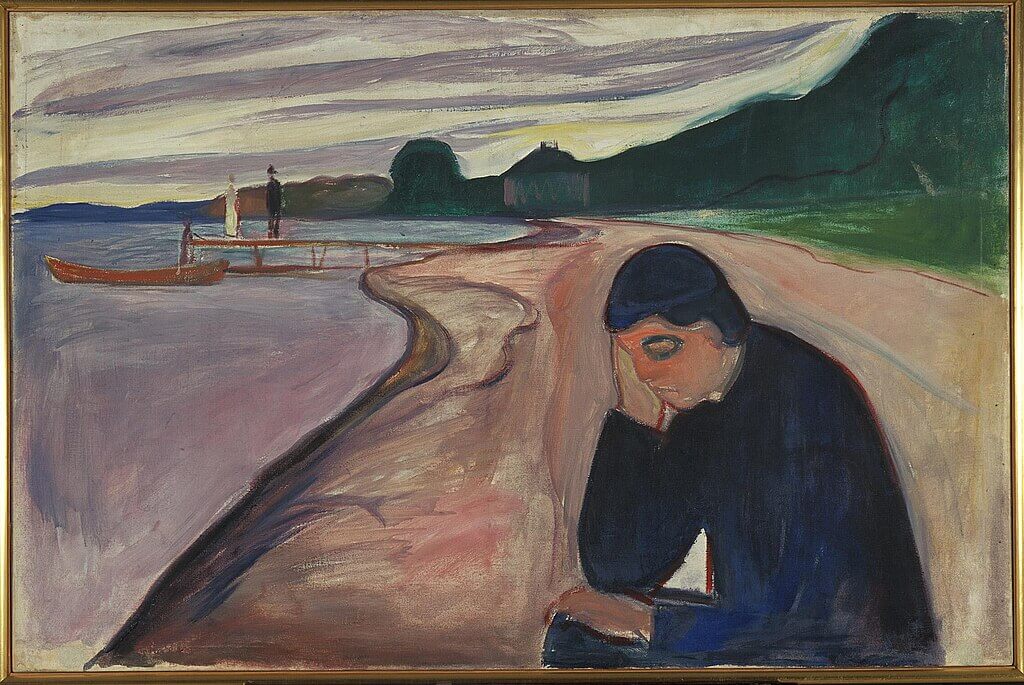
Edvard Munch painting
Edvard Munch, CC BY-SA 4.0 https://creativecommons.org/licenses/by-sa/4.0, via Wikimedia Commons

The moment of death

The death scene is restrained, without emphasis, but devastating:

«Le bruit de l’oxygène s’était tu, le médecin s’éloigna du lit. Ma grand’mère était morte.»

“The sound of oxygen had fallen silent, the doctor moved away from the bed. My grandmother was dead.”

Immediately after death, the grandmother’s face undergoes a transfiguration: it becomes younger, purified. Proust describes how she appears as she did when her parents were choosing her husband, her features radiating hope and innocence:

«Elle avait les traits […] brillantes d’une chaste espérance, d’un rêve de bonheur, même d’une innocente gaieté, que les années avaient peu à peu détruits.»

“She had features […] bright with a chaste hope, a dream of happiness, even an innocent gaiety, that the years had gradually destroyed.”

The body reveals an image of her that time had gradually erased. Death, paradoxically, becomes a moment of identity revelation—uncovering the true self that had been obscured by the passing years.

The impact on the narrator’s consciousness

The grandmother’s death marks a decisive end to the narrator’s emotional childhood. This profound loss triggers several far-reaching consequences:

  1. A visceral understanding of time’s irreversibility.
  2. The shattering of emotional illusions (the realization that nothing lasts forever).
  3. A deep crisis of confidence in both language and appearances.
  4. Recognition of the body’s mortality and society’s pretenses.
  5. The awakening of his literary vocation as a means to preserve memory.

Later, the narrator will see his grandmother’s features reflected in his mother’s face—a testament to how memory lives on through physical resemblance and inner perception.

Narrative techniques

The passages depicting the grandmother’s illness and death showcase Proust’s exceptional artistic prowess. In portraying this tragic event, he employs several sophisticated narrative techniques:

  • Perceptual shift: Rather than presenting the illness as a sudden, clear occurrence, Proust reveals it through a gradual process of understanding based on subtle changes in gestures, facial expressions, and behavior.
  • Poetic objectification: Ordinary objects transform into powerful symbols—notably the thermometer, which becomes a witch or prophetess capable of revealing truths that doctors cannot recognize.
  • Internal focalization: All events are filtered exclusively through the narrator’s consciousness, revealing his dismay, pain, confusion, and helplessness.
  • Manipulation of narrative time: Brief moments expand into extensive, meaning-rich descriptions. Proust creates a divergence between real time and psychological time, producing a deceleration that suspends expectation and extends the perception of suffering.

Parallels with other authors

The portrayal of illness as revelation echoes throughout contemporary European literature:

  • Tolstoy (The Death of Ivan Ilyich): suffering strips away bourgeois pretensions, revealing essential truths.
  • Thomas Mann (The Magic Mountain): the sanatorium becomes a liminal space where time suspends, allowing deep existential contemplation.
  • Virginia Woolf (On Being Ill): illness emerges as both a subjective experience and an unacknowledged language within literature.
  • Mikhail Bulgakov (A Young Doctor’s Notebook): the doctor exists in a vulnerable state between technical knowledge and human limitations, confronting mortality’s inevitability.

For these authors, as for Proust, illness transcends its biological dimensions to become a threshold revealing existential truth.

Conclusion

The grandmother’s death in the Recherche represents one of literature’s most profound portrayals of illness as both crisis and revelation. Through this suffering, the narrator undergoes a transformative experience that leads him to comprehend the redemptive power of memory and writing. Medicine appears in this narrative not just as powerless, but as tragically blind to what body and soul wordlessly express. From this silence emerges literature itself.

Children splash and play in a shallow forest river around a bright blue whale-shaped toy boat, while a large container ship labeled “docker” looms in the background, all rendered in a warm, nostalgic painterly style.

Create a Medical Database with Docker: Complete Guide with SQLAlchemy, and Flask

Posted on July 1, 2025August 11, 2026 by Michele Danilo Pierri

Introduction: Why Build a Medical Database with Docker?

Creating a robust medical database system requires careful consideration of security, scalability, and maintainability. Furthermore, Docker containerization offers an ideal solution for healthcare applications by providing isolated environments that ensure consistent deployment across different systems.

In this comprehensive tutorial, we’ll explore how to create a medical database with Docker and perform operations on it using various tools. Additionally, we’ll use a practical example: a database designed to store patient demographic and anthropometric data (age, sex, height, weight, etc.).

While the structure we present is relatively simple, it can be scaled to accommodate more complex architectures. Moreover, this foundation provides the flexibility needed for future healthcare system expansions.

Table of Contents

Introduction

  • Overview of the tutorial
  • Purpose and scope

Tools We’ll Use

  • Docker
    • Overview and containerization
    • Benefits of isolation
    • MySQL container setup
  • SQLAlchemy
    • Database interaction capabilities
    • ORM functionality
  • Flask
    • Web framework basics
    • Database interface creation

Step-by-Step Guide

  • Step 1: Download and Configure MySQL Container
    • Docker installation
    • Container configuration
    • Basic Docker commands
  • Step 2: Creating Tables with SQLAlchemy
    • Database structure setup
    • Table relationships
    • Data modeling
  • Step 3: Data Operations with SQLAlchemy
    • Session management
    • Data insertion
    • Query operations
  • Step 4: Web Interface with Flask
    • Application setup
    • Route definitions
    • Template organization
  • Step 5: Security Consideration
  • Step 6: Summary

All the code for this project is available on GitHub


Essential Tools for Medical Database Development

Why Docker Transforms Healthcare Database Management

Building a medical database with Docker provides several advantages including isolation, portability, and ease of setup. First of all, Docker is an open-source tool for developing, distributing, and running software.

Its key feature is containerization—applications run in isolated environments that contain everything needed for the program to work. However, these containers share the host computer’s kernel while remaining isolated from its operating system. Think of them as lightweight virtual machines that are more efficient because they leverage the host’s kernel.

Thanks to isolation from the “host” environment, containers prevent conflicts from different dependencies and configurations. Consequently, they operate independently from the system while maintaining data persistence through mounted volumes.

SQLAlchemy: Simplifying Database Interactions

Next, SQLAlchemy is one of the most popular Python libraries for working with relational databases. It enables Python code to interact directly with various SQL databases through specific drivers, including MySQL, PostgreSQL, Oracle, and SQLite.

A key feature of SQLAlchemy is its Object-Relational Mapper (ORM), which maps database tables to Python classes. As a result, database interactions become straightforward and intuitive, reducing development time significantly.

Flask: Creating User-Friendly Web Interfaces

Flask is a Python framework for creating web applications. With Flask, we can build SQLAlchemy applications that access databases through an HTML interface. Therefore, users can interact with the medical database without requiring technical database knowledge.

Prerequisites

To start the project, you need Docker (available at Docker: Accelerated Container Application Development) and Python (Download Python | Python.org) installed on your computer.

Step 1: Download and Configure MySQL Container

Setting Up Your Docker Environment

With Docker running on your computer, you can download the MySQL database image from the terminal using this command:

docker pull mysql:latest

This command downloads the latest MySQL image from the Docker Hub repository. Subsequently, once the image download is complete, we can create a container from it and configure it to meet our requirements.

Container Configuration and Setup

Navigate to the directory where you want to store your database (using standard commands like cd and mkdir). Then, run this script in the terminal:

docker run --name my-mysql-container \\
	-v my_directory/data:/var/lib/mysql \\ 
  -e MYSQL_ROOT_PASSWORD=my-secret-pw \\
  -e MYSQL_DATABASE=mydatabase \\
  -e MYSQL_USER=myuser \\
  -e MYSQL_PASSWORD=mypassword \\
  -p 3306:3306 \\
  -d mysql:latest

Here’s what each parameter means:

  • –name: Sets the container’s name for easy identification
  • -v: Specifies the volume where data is stored, ensuring persistence
  • -e: Defines environment variables, including database credentials
  • -p: Specifies communication ports for external access
  • -d: Runs the container in detached mode

Managing Container Operations

These commands are only needed when initializing the container for the first time. After that, the specified parameters are saved and automatically applied whenever you run the container.

To verify the program has started successfully, use:

docker ps

Once you’ve created and configured the container, you won’t need to use docker run again. Instead, you’ll use different commands to stop and restart the program.

Furthermore, to manage your container operations use:

To stop the container:

docker stop my-mysql-container

To restart it, use:

docker start my-mysql-container

To completely delete the container, use this command:

docker rm -f my-mysql-container

Note: An alternative method called docker compose lets you manage container configurations through a docker-compose.yml file. This approach is typically used for applications with multiple containerized programs, but we won’t cover it in this tutorial.

Step 2: Creating Database Tables with SQLAlchemy

Environment Setup and Library Installation

It is recommended to use an IDE (like Visual Studio Code) and create a virtual environment to complete this step; you also need to verify that the container is active or activate it with the command:

docker start my-mysql-container

From Visual Studio Code’s terminal, install the required Python libraries:

pip install sqlalchemy pymysql

Establishing Database Connection

From Python, let’s import the required libraries:

from sqlalchemy import create_engine, Column, Integer, String, Date, Float, ForeignKey
from sqlalchemy.ext.declarative import declarative_base
from sqlalchemy.orm import sessionmaker, relationship

Define the database connection string (Replace ‘myuser’, ‘mypassword’, ‘localhost’, and ‘mydatabase’ with your actual MySQL credentials)

DATABASE_URL = "mysql+pymysql://myuser:mypassword@localhost:3306/mydatabase"

Create an engine to connect to the database. The engine manages the connection pool and database access. Setting echo=True enables SQL statement logging for debugging.

engine = create_engine(DATABASE_URL, echo=True) 

SQLAlchemy uses a foundational “base” class that helps create database tables in Python. This base class acts as a template – when you create new table classes, they inherit from this base class, making it simple to define and work with database tables in your Python code.

To define it, we use the command:

Base = declarative_base()

Designing Patient Records Table

Now let’s create the first table, the patient’s PatientRecords using SQLAlchemy’s Base class as a template:


class PatientRecords(Base):
    __tablename__ = 'patient_records'  # Table name in the database

    # Columns
    Id_patient = Column(Integer, primary_key=True, autoincrement=True)  # Primary key
    first_name = Column(String(50), nullable=False)  # Patient's first name
    last_name = Column(String(50), nullable=False)  # Patient's last name
    date_of_birth = Column(Date, nullable=False)  # Patient's date of birth

    # Relationship with the "AnthropometricData" table
    anthropometric_data = relationship("AnthropometricData", back_populates="patient")

    def __repr__(self):
        return f"<PatientRecords(Id_patient={self.Id_patient}, first_name={self.first_name}, last_name={self.last_name})>"

In this script, we define both the table name (patients_record) and its fields, while also establishing a relationship with the Anthropometric_data table (relationship = AnthropometricData). This relationship is bidirectional (back_populates = “patient”). When we create the Anthropometric_data table, we’ll set up a corresponding PatientRecord relationship with a bidirectional link (back_populates = AnthropometricData) to the Patient_record table.

This creates a “logical” link between the two tables, complementing the structural connection already established through Foreign Keys at the database level.

The repr(self) method defines how an object should be represented when it is printed or displayed, converting it into a more readable string format.

Creating Anthropometric Data Table

Let’s create the second table (antropometric_data) using the same approach we used for the PatientRecords table.

class AnthropometricData(Base):
    __tablename__ = 'anthropometric_data'  # Table name in the database

    # Columns
    Id_data = Column(Integer, primary_key=True, autoincrement=True)  # Primary key
    Id_patient = Column(Integer, ForeignKey('patient_records.Id_patient'), nullable=False)  # Foreign key to "patient_records"
    height = Column(Float, nullable=False)  # Height in cm
    weight = Column(Float, nullable=False)  # Weight in kg
    BMI = Column(Float, nullable=False)  # Body Mass Index (calculated as weight / (height/100)^2)

    # Relationship with the "PatientRecords" table
    patient = relationship("PatientRecords", back_populates="anthropometric_data")

    def __repr__(self):
        return f"<AnthropometricData(Id_data={self.Id_data}, Id_patient={self.Id_patient}, BMI={self.BMI})>"

It’s important to note that, at this point, the tables exist only as logical definitions and haven’t been created in the actual database. The following command will transform them into real tables in our archive by converting our logical structure into SQL commands. SQLAlchemy handles this conversion automatically, saving us significant effort.

Base.metadata.create_all(engine)

To verify that the tables were successfully created, you can interact directly with the MySQL database through the terminal with these commands:

docker exec -it my-mysql-container mysql -u myuser -p
USE mydatabase;
SHOW TABLES;
DESCRIBE patient_records;
DESCRIBE anthropometric_data;

These commands will display the following:

command SHOW TABLES

SQL command DESCRIBE patients_records

SQL command DESCRIBE anthropometric_data

Step 3: Data Operations and Management

Session Management and Database Operations

After setting up the database and tables, we can proceed to populate them with content.

If you create a new program to perform database operations, you’ll need to include the table class definitions (PatientRecords and AnthropometricData) again. While you can copy these definitions manually, there are more efficient ways to avoid this duplication, though we’ll keep things simple and won’t cover those techniques here.

In order to perform database operations (such as queries and data insertion) with SQLAlchemy, we first need to use sessionmaker.

Session = sessionmaker(bind=engine)
session = Session()

When creating a session using sessionmaker, these operations happen automatically:

  • Connection to the database through the engine
  • Tracking of all pending database operations
  • Execution of all operations in a single block when committed

A session follows this lifecycle:

  • Creation (session = Session())
  • Database interactions (queries, reads, insertions)
  • Saving changes (session.commit())
  • Rolling back changes if errors occur (session.rollback())
  • Closing the session (session.close())

Adding Patient Records

Now that we have created a session, we can add a new patient to the patient_records table:

new_patient = PatientRecords(
    first_name="Mario",
    last_name="Rossi",
    date_of_birth="1990-05-15"  # Date format: YYYY-MM-DD
)
session.add(new_patient)
session.commit()

Note that we insert the new patient using the Python table class (PatientRecords) rather than the actual table name (patient_records). SQLAlchemy provides this layer of abstraction, letting us focus on logical operations instead of directly referencing table names. Behind the scenes, SQLAlchemy converts our code into SQL instructions to interact with the database.

Managing Anthropometric Data

Next, let’s add data to the anthropometric_data table:

anthropometric_data = AnthropometricData(
    Id_patient=new_patient.Id_patient,
    height=175.0,  # Height in cm
    weight=70.0,   # Weight in kg
    BMI=70.0 / ((175.0 / 100) ** 2)  # Calculate BMI
)
session.add(anthropometric_data)
session.commit()

Querying and Verification

Let’s query the tables to verify that our data was successfully inserted:


patients = session.query(PatientRecords).all()
print("\\nPatients in the database:")
for patient in patients:
    print(patient)

anthropometric_records = session.query(AnthropometricData).all()
print("\\nAnthropometric Data in the database:")
for record in anthropometric_records:
    print(record)

Finally, let’s close the session:

session.close()

Alternatively, you can query the database directly through Docker using SQL commands in the terminal:

docker exec -it my-mysql-container mysql -u myuser -p
USE mydatabase;
SELECT * FROM patient_records;
SELECT * FROM anthropometric_data;

The terminal will display the following results:

SQL command SELECT * FROM

Step 4: Building a Web Interface with Flask

Flask Installation and Setup

Flask is a lightweight web framework that lets you create browser-accessible applications to interact with MySQL containers.

First, install Flask in Python by running this command in the terminal:

pip install Flask

Next, we need to create a file called models.py that reuses our previous ORM class definitions for the database tables:

from sqlalchemy import Column, Integer, String, Date, Float, ForeignKey
from sqlalchemy.ext.declarative import declarative_base
from sqlalchemy.orm import relationship

Base = declarative_base()

class PatientRecords(Base):
    __tablename__ = 'patient_records'

    Id_patient = Column(Integer, primary_key=True, autoincrement=True)
    first_name = Column(String(50), nullable=False)
    last_name = Column(String(50), nullable=False)
    date_of_birth = Column(Date, nullable=False)

    anthropometric_data = relationship("AnthropometricData", back_populates="patient")

    def __repr__(self):
        return f"<PatientRecords(Id={self.Id_patient}, Name={self.first_name} {self.last_name})>"

class AnthropometricData(Base):
    __tablename__ = 'anthropometric_data'

    Id_data = Column(Integer, primary_key=True, autoincrement=True)
    Id_patient = Column(Integer, ForeignKey('patient_records.Id_patient'), nullable=False)
    height = Column(Float, nullable=False)
    weight = Column(Float, nullable=False)
    BMI = Column(Float, nullable=False)

    patient = relationship("PatientRecords", back_populates="anthropometric_data")

    def __repr__(self):
        return f"<AnthropometricData(Id={self.Id_data}, PatientId={self.Id_patient}, BMI={self.BMI})>"

Finally, we can create an app.py using Flask.

Our medical database project will use three HTML templates as the foundation for interacting with the container:

  • index.html – the main page
  • add_patient.html – for adding new patients
  • edit_patient.html – for modifying patient records

Directory Structure and Organization

The directory organization will be:

flask_app/
│
├── app.py               # Main Flask app file
├── models.py            # ORM class definitions (PatientRecords, AnthropometricData)
├── templates/           # HTML templates folder
│   ├── index.html       # Main page
│   ├── add_patient.html # Form to add a patient
└   └── edit_patient.html# Form to modify a patient

We’ll create three HTML templates. The first (index.html) serves as the entry page, displaying the database content and allowing users to select various operations.

The second page (add_patient.html) provides a form for adding patients to the patient_records dataset, while the third page (edit_patient.html) enables modification of existing patient data.

At this stage, we’ve prioritized system functionality over aesthetics, though the visual aspects can be easily improved later.

The script for index.html:

<!DOCTYPE html>
<html>
<head>
    <title>Patient List</title>
</head>
<body>
    <h1>Patient List</h1>
    <!-- Link to add a new patient -->
    <a href="{{ url_for('add_patient') }}">Add New Patient</a>
    <ul>
        <!-- Loop through all patients and display their details -->
        {% for patient in patients %}
            <li>
                {{ patient.first_name }} {{ patient.last_name }}
                <!-- Links to edit or delete the patient -->
                (<a href="{{ url_for('edit_patient', patient_id=patient.Id_patient) }}">Edit</a> |
                <a href="{{ url_for('delete_patient', patient_id=patient.Id_patient) }}">Delete</a>)
            </li>
        {% endfor %}
    </ul>

The script for add_patient.html:

<!DOCTYPE html>
<html>
<head>
    <title>Add Patient</title>
</head>
<body>
    <h1>Add a New Patient</h1>
    <!-- Form to submit new patient details -->
    <form method="POST">
        First Name: <input type="text" name="first_name"><br>
        Last Name: <input type="text" name="last_name"><br>
        Date of Birth: <input type="date" name="date_of_birth"><br>
        <button type="submit">Add Patient</button>
    </form>
    <!-- Link to return to the patient list -->
    <a href="{{ url_for('index') }}">Back to Patient List</a>
</body>
</html>

The script for edit_patient.html:

<!DOCTYPE html>
<html>
<head>
    <title>Edit Patient</title>
</head>
<body>
    <h1>Edit Patient Details</h1>
    <!-- Form to update patient details -->
    <form method="POST">
        First Name: <input type="text" name="first_name" value="{{ patient.first_name }}"><br>
        Last Name: <input type="text" name="last_name" value="{{ patient.last_name }}"><br>
        Date of Birth: <input type="date" name="date_of_birth" value="{{ patient.date_of_birth }}"><br>
        <button type="submit">Save Changes</button>
    </form>
    <!-- Link to return to the patient list -->
    <a href="{{ url_for('index') }}">Back to Patient List</a>
</body>
</html>

Flask Application Development

The app.py program follows below. The program uses Flask decorators (marked by “@app.route()”) to connect web pages with Python code, managing database requests and responses.

from flask import Flask, render_template, request, redirect, url_for
from sqlalchemy import create_engine
from sqlalchemy.orm import sessionmaker
from models import PatientRecords, AnthropometricData

# Database configuration
DATABASE_URL = "mysql+pymysql://myuser:mypassword@localhost:3306/mydatabase"
engine = create_engine(DATABASE_URL)  # Create a connection to the database
Session = sessionmaker(bind=engine)  # Create a session factory
session = Session()  # Initialize a session to interact with the database

# Initialize Flask app
app = Flask(__name__)

# Home Page: Display all patients
@app.route("/")
def index():
    patients = session.query(PatientRecords).all()  # Query all patients from the database
    return render_template("index.html", patients=patients)  # Render the template with patient data

# Add Patient Page: Handle form submission to add a new patient
@app.route("/add", methods=["GET", "POST"])
def add_patient():
    if request.method == "POST":
        # Retrieve form data
        first_name = request.form["first_name"]
        last_name = request.form["last_name"]
        date_of_birth = request.form["date_of_birth"]

        # Create a new patient object
        new_patient = PatientRecords(
            first_name=first_name,
            last_name=last_name,
            date_of_birth=date_of_birth
        )
        session.add(new_patient)  # Add the new patient to the session
        session.commit()  # Commit the transaction to save the data
        return redirect(url_for("index"))  # Redirect to the home page
    return render_template("add_patient.html")  # Render the form for GET requests

# Edit Patient Page: Handle form submission to update an existing patient
@app.route("/edit/<int:patient_id>", methods=["GET", "POST"])
def edit_patient(patient_id):
    patient = session.query(PatientRecords).get(patient_id)  # Retrieve the patient by ID
    if request.method == "POST":
        # Update patient details with form data
        patient.first_name = request.form["first_name"]
        patient.last_name = request.form["last_name"]
        patient.date_of_birth = request.form["date_of_birth"]
        session.commit()  # Commit the changes to the database
        return redirect(url_for("index"))  # Redirect to the home page
    return render_template("edit_patient.html", patient=patient)  # Render the edit form

# Delete Patient Page: Delete a patient by ID
@app.route("/delete/<int:patient_id>")
def delete_patient(patient_id):
    patient = session.query(PatientRecords).get(patient_id)  # Retrieve the patient by ID
    session.delete(patient)  # Delete the patient from the session
    session.commit()  # Commit the transaction to apply the deletion
    return redirect(url_for("index"))  # Redirect to the home page

# Run the Flask app
if __name__ == "__main__":
    app.run(debug=True)  # Start the app in debug mode for development

The initial page displays the database records and all available actions that can be performed on them:

Patient list

The additional pages enable users to add or modify patient records:

Add a new patient

Edit Patient Details

Step 5: Critical Security Considerations

Understanding Healthcare Data Protection

We are dealing with a medical database and therefore sensitive data whose protection is regulated by legislation. Moreover, GDPR (General Data Protection Regulation) in Europe and HIPAA (Health Insurance Portability and Accountability Act) in the United States impose strict requirements.

Identifying Security Vulnerabilities

Even with a superficial analysis, we can identify numerous critical issues in the structure we have built:

  • Exposed passwords: Access credentials to the dataset are embedded in the code and therefore easily stolen.
  • Unauthenticated access: The Flask application lacks authentication mechanisms for HTML pages.
  • Unencrypted data: Data transmission between the Flask server and HTML pages is not encrypted.
  • SQL injection vulnerability: Input data is not validated, exposing the system to attacks through harmful SQL commands.
  • Cross-Site scripting vulnerability: Malicious users could exploit the web interface to inject harmful scripts.
  • Database exposure: The database is accessible on port 3306: if this port is public, it could be targeted for direct attacks.

Implementing Security Measures

Solutions to these issues include:

  • Environment variable management for credentials
  • Authentication middleware implementation
  • HTTPS encryption for data transmission
  • Input validation and parameterized queries
  • Content Security Policy headers
  • Network segmentation and firewall rules

Step 6: Summary and Next Steps

Key Concepts Review

Let’s summarize the key concepts covered in this tutorial:

First, we used Docker to create a MySQL container, providing an isolated and configurable medical database environment. Subsequently, we implemented SQLAlchemy as an ORM to map database tables to Python classes. Finally, we built a Flask web application that enables browser-based database interactions.

Future Development Possibilities

While this structure is straightforward, it serves as a robust foundation. Furthermore, it can be expanded into more complex architectures including:

  • Multi-container orchestration with Docker Compose
  • Advanced authentication and authorization systems
  • Real-time data synchronization capabilities
  • Comprehensive audit logging mechanisms
  • Integration with Electronic Health Record (EHR) systems

Scaling Considerations

As your medical database grows, consider implementing:

  • Database indexing strategies for improved performance
  • Caching mechanisms for frequently accessed data
  • Load balancing for high-availability deployments
  • Backup and disaster recovery procedures
  • Compliance monitoring and reporting tools

Conclusion: Building Secure Healthcare Systems

This tutorial has provided a comprehensive foundation for building medical databases with Docker. However, remember that production healthcare systems require additional security measures and compliance considerations.

Therefore, always consult with security professionals and legal experts when handling sensitive medical data. Additionally, stay updated with the latest security best practices and regulatory requirements in your jurisdiction.

A physician in an early 20th-century radiology room examines a chest X-ray displayed on an illuminated viewing panel, surrounded by vintage medical equipment.

UNet

Posted on May 4, 2025August 11, 2026 by Michele Danilo Pierri

Introduction

UNet is a convolutional neural network (CNN) introduced by Olaf Ronneberger in 2015. These specialized neural networks learn to recognize objects in images. When properly trained, they can analyze medical images, detect specific features (such as neoplasms in CT scans), and classify different types of images (such as distinguishing between pneumonia and neoplasms).

In particular, UNet performs semantic interpretation of images by identifying and classifying pixels. It was specifically designed for medical applications and has the advantage of working effectively with small datasets.

UNet Anatomy

The UNet architecture consists of two joined arms that form a U-like shape: a left Encoder arm that extracts significant features from an image, and a right Decoder arm that reconstructs the image using the extracted information. Skip Connections between the arms link corresponding layers of the Encoder and Decoder, helping maintain spatial details.

UNet Architecture Diagram

Encoder Structure

The encoder consists of 4 levels. Each level includes:

  • two Convolutional Blocks
  • a Max Pooling layer
  • a channel multiplier (filter)

Level of Encoder

The first convolutional block examines images pixel by pixel to detect patterns like corners and shapes. They do this by sliding a 3 × 3 filter (kernel) across the image, multiplying pixel values by filter weights and summing the results at each position.

The first convolutional block applies sixty-four 3×3 filters to the image.

This process creates a “feature map” that summarizes all recognized patterns in the image.

For example, when searching for edges and lines, they will be highlighted in the feature map once the convolutional block is processed.

After convolution, a ReLU (Rectifier Linear Unit) function is applied that converts all negative values to 0 while preserving positive values.

The second convolutional block repeats this process with another filter, creating more complex structures from the patterns identified in the first block. For instance, while the first block detects edges and lines, the second block combines these elements into shapes like circles and rectangles.

After the second convolutional block, the Max Pooling layer reduces the dimensions by 50%.

Through this process, the initial 572 × 572 pixel image is transformed by 64 3 × 3 filters into a 570 × 570 × 64 array. The second convolution with a 3 × 3 filter transforms the image to 568 × 568 pixels, and then the Max Pooling reduces it to 284 × 284 × 64 before proceeding to the next block.

Subsequent Encoder Levels

Through this process, at the first level of Encoder the initial 572 × 572 pixel image is transformed by 64 3 × 3 filters into a 570 × 570 × 64 array. The second convolution with a 3 × 3 filter transforms the image to 568 × 568 pixels, and then the Max Pooling reduces it to 284 × 284 × 64 before proceeding to the next block.

The subsequent levels (second, third, and fourth) mirror the first level’s structure. Each consists of two successive 3 × 3 convolutional blocks followed by Max Pooling. As each convolutional block introduces new filters, this process progressively reduces the image’s pixel dimensions while increasing the number of channels (filters).

Summary of Encoder Modifications

(Starting with a 572 × 572 × 1 grayscale image)

LevelOperationChannelImage Pixel
I2 convolutional block 3×3 and 1 max pooling 2 x264572 x 572
2 convolutional block 3×3 and 1 max pooling 2 x2128284 x 284
III2 convolutional block 3×3 and 1 max pooling 2 x2256140 x 140
IV2 convolutional block 3×3 and 1 max pooling 2 x251270 x 70 to 34 x 34

As the image progresses through different levels, its content becomes increasingly abstract and concentrated. At the first level, the network detects simple features like edges and corners. These basic elements combine into shapes at the second level, evolve into more complex structures (such as textures and object parts) at the third level, and finally transform into overall semantic meaning at the fourth level. This increasing complexity corresponds directly with the growing number of channels.

Bottleneck

The bottleneck serves as the final part of the Encoder process and bridges the Encoder and Decoder. It receives the minimally reduced image with maximum channels from the Encoder and applies two additional 3 × 3 convolutional blocks without Max Pooling before transferring it to the Decoder.

During this process, the number of channels increases to 1024.

At this stage, the image reaches its most compressed form.

The first convolutional block reduces the image to 32 × 32 pixels, while the second block further compresses it to 30 × 30 pixels.

The final Bottleneck output is a 30 × 30 pixel image with 1024 channels.

Level of Decoder

The Decoder, which forms UNet’s “ascending” branch, consists of 4 identical blocks.

Each block performs a sequence of operations: upsampling, concatenation, and two convolutions.

Upsampling increases the feature map dimensions from the Bottleneck’s minimum 30 × 30 pixels. This process uses a 2 × 2 transposed convolution kernel to expand the dimensions. In the first block, upsampling takes a 30 × 30 pixel image with 1024 channels and produces a 62 × 62 pixel image with 514 channels.

Upsampling serves two main purposes:

  • It reconstructs images by recovering details lost during the encoder process
  • It aligns the feature map dimensions with the corresponding encoder level to enable concatenation via skip connections

After upsampling, the image is concatenated with its corresponding image from the homologous encoder block through the skip connection, joining them along the channel dimension.

The image from the last Encoder block (70 × 70 × 514 channels) is cropped to match the Decoder’s dimensions.

The dimensions combine as follows:

62 x 62 x 514 (Encoder) + 62 x 62 x 514 (Decoder) = 62 x 62 x 1024

Finally, the concatenated image undergoes two 3 × 3 convolutions, reducing it to the first decoder level’s output dimensions of 62 × 62 × 514.

Subsequent Decoder Levels

If the first level, with upsampling operations, concatenation and double convolution brings the image from the bottleneck to dimensions of 62 x 62 x 514, in the subsequent Decoder levels, all identical, the images are increased until reaching final dimensions of 464 x 464 x 64 at the end of the last stage

Summary of Decoder Modifications

LEVEL1234
DECODER INPUT30×30×102458×58×512116×116×256232×232×128
UPSAMPLING62×62×512120×120×256236×236×128468×468×64
SKIP CONNECTION62×62×512120×120×256236×236×128468×468×64
CONCATENATION62×62×1024120×120×512236×236×256468×468×128
AFTER CONVOLUTIONS58×58×512116×116×256232×232×128464×464×64

After the final Decoder stage, the network applies a 1×1 convolution followed by an activation function (either SoftMax or sigmoid) to calculate the probability for each pixel.

The final output is a 464×464 image.

Architectural Overview

INPUT: 572x572x1
│
├── Encoder
│   ├── Conv(3x3, 64) → ReLU → Conv(3x3, 64) → ReLU → MaxPool(2x2)
│   ├── Conv(3x3, 128) → ReLU → Conv(3x3, 128) → ReLU → MaxPool(2x2)
│   ├── Conv(3x3, 256) → ReLU → Conv(3x3, 256) → ReLU → MaxPool(2x2)
│   └── Conv(3x3, 512) → ReLU → Conv(3x3, 512) → ReLU → MaxPool(2x2)
│
├── Bottleneck
│   └── Conv(3x3, 1024) → ReLU → Conv(3x3, 1024) → ReLU → UpConv(2x2)
│
└── Decoder
    ├── Concatenate(UpConv, Encoder[4]) → Conv(3x3, 512) → ReLU → Conv(3x3, 512) → ReLU → UpConv(2x2)
    ├── Concatenate(UpConv, Encoder[3]) → Conv(3x3, 256) → ReLU → Conv(3x3, 256) → ReLU → UpConv(2x2)
    ├── Concatenate(UpConv, Encoder[2]) → Conv(3x3, 128) → ReLU → Conv(3x3, 128) → ReLU → UpConv(2x2)
    └── Concatenate(UpConv, Encoder[1]) → Conv(3x3, 64) → ReLU → Conv(3x3, 64) → ReLU
│
└── Output: Conv(1x1, C) → Sigmoid/Softmax

UNet Results

UNet generates a “segmentation map” (called a Mask) rather than returning a copy of the input image. This Mask highlights structures of interest by assigning numerical values to each pixel.

The Mask maintains the same dimensions as the original image, with pixel values varying based on the classification task:

  • In binary classification, pixels get a value of 1 for the structure of interest and 0 for everything else
  • In multiclass classification, pixels receive values corresponding to their class (1 for the first class, 2 for the second class, 0 for background)

For example, when UNet is trained to detect tumors, the Mask marks tumor pixels with 1 and non-tumor pixels with 0.

We can visualize the tumor’s location by overlaying this mask on the original image.

UNet Evaluation Metrics

The quality of results obtained by UNet can be evaluated using different metrics:

Dice Coefficient

The Dice Coefficient can be compared to the F1 score for images.

A Dice Coefficient equal to one indicates a perfect map.

Considering P as the predicted map and G as the ground truth map, the dice coefficient is:

\text{Dice} = \frac{2 \cdot |P \cap G|}{|P| + |G|}

Intersection over Union (IoU)

Another metric is the Intersection over Union which also classifies a perfect map as 1. Unlike the Dice coefficient, IoU (Jaccard Index) is more sensitive to small differences

\text{IoU} = \frac{|P \cap G|}{|P \cup G|} = \frac{|P \cap G|}{|P| + |G| - |P \cap G|}

Accuracy

Measures the percentage of correctly classified pixels

Precision/recall

Ability to recognize true positives without false positives.

Challenges When Using UNet

The first challenge is dimensional discrepancy between input and output images. Without proper corrections, the output image becomes smaller than the input. This can be resolved by applying padding to the convolutions or by upscaling the final result.

The second challenge is overfitting, where the model becomes too specialized to its training examples. This is addressed through data augmentation techniques.

The third challenge is class imbalance, particularly common in biomedical data. For instance, a tumor might occupy only a small portion of the image’s pixels. To handle this, specialized loss functions like Dice Loss or Focal Loss are implemented.

Applications of UNet in Medicine

There are examples of UNet applications in the medical field:

Walsh J – Using U-Net network for efficient brain tumor segmentation in MRI images – https://doi.org/10.1016/j.health.2022.100098**

Hassanpour N, Deep Learning-based Bio-Medical Image Segmentation using UNet Architecture and Transfer Learning – https://doi.org/10.48550/arXiv.2305.14841

Ehab W – Performance Analysis of UNet and Variants for Medical Image Segmentation – https://doi.org/10.48550/arXiv.2309.13013

Further Readings

The original work where Ronneberger shared the UNet architecture can be found at https://doi.org/10.48550/arXiv.1505.04597

U-Net Image Segmentation in Keras U-Net Image Segmentation in Keras – PyImageSearch

PyTorch UNet https://github.com/milesial/Pytorch-UNet

UNet Architecture explained: U-Net Architecture Explained | GeeksforGeeks

Conclusion

UNet has established itself as a foundational standard in contemporary biomedical research and clinical applications. Its widespread adoption and continued success can be attributed to several key capabilities that make it particularly valuable in medical image analysis:

  • Preserve spatial details with high fidelity (through its innovative skip connections architecture), allowing it to maintain crucial anatomical information and subtle features that are essential for accurate medical diagnosis and analysis.
  • Adapt seamlessly to diverse data modalities (including MRI, CT, microscopic images, ultrasounds, and X-rays), demonstrating remarkable versatility across different medical imaging technologies and protocols while maintaining consistent performance.
  • Support continuous evolution through advanced variants (such as 3D UNet for volumetric analysis, Attention UNet for focused feature detection, and UNet++ for enhanced precision), enabling researchers to build upon its robust foundation to address increasingly complex medical imaging challenges.
  • Deliver reliable performance even with limited training data, making it particularly valuable in medical contexts where large annotated datasets are often difficult to obtain.
  • Maintain computational efficiency while processing high-resolution medical images, enabling practical implementation in clinical settings where rapid analysis is crucial.
A group of barefoot children in worn old-fashioned clothes stands on a stormy beach, holding seashells to their ears as they gaze toward the sea and dramatic rays of sunlight breaking through heavy clouds above crashing waves.

Sensitivity Analysis

Posted on April 4, 2025August 2, 2026 by Michele Danilo Pierri

Definition

Sensitivity analysis is a collection of techniques that determine how input parameters affect model results. Specifically, it measures how much variation in the results stems from different types of uncertainty.

For a model:

Y=f(X_1,X_2,X_3…..X_n)

examines how Y changes when each X is modified.

Sensitivity analysis can be applied across several key areas: predictive models, simulation, risk assessment, complex systems optimization, model validation.

Through sensitivity analysis, we can evaluate how variables affect outputs, simplify models by identifying negligible variables, pinpoint the most influential factors, and increase the transparency of model evaluation.

Sensitivity Analysis Techniques

Here are the main sensitivity analysis techniques we will explore:

One-at-a-Time (OAT)

Sobol Analysis

FAST

Regression-based (SRC, PCC)

SHAP Values

Random Forest Feature Importance

Tornado Plot

Bayesian Sensitivity (PyMC, Prob. Mod.)

DoE + ANOVA

One At a Time (OAT)

This technique involves changing one input variable at a time while keeping all others constant, then measuring how the output changes.

While simple to implement, this technique has limitations: it may overlook non-linear relationships and, crucially, fails to capture interactions between variables.ired for security purposes.

import numpy as np
import matplotlib.pyplot as plt

# Define a simple model (nonlinear)
def model(x):
    """x = [x1, x2, x3]"""
    return np.sin(x[0]) + 0.5 * x[1]**2 + np.log1p(x[2])

# Baseline input
x_base = np.array([1.0, 2.0, 3.0])
y_base = model(x_base)

# Define perturbation (e.g., ±10%)
delta = 0.1

# Store results
sensitivities = []
labels = ['x1', 'x2', 'x3']

for i in range(len(x_base)):
    x_perturb = x_base.copy()
    x_perturb[i] *= (1 + delta)  # increase by 10%
    y_perturb = model(x_perturb)
    sensitivity = (y_perturb - y_base) / (x_perturb[i] - x_base[i])  # finite difference
    sensitivities.append(sensitivity)

# Plot results
plt.bar(labels, sensitivities)
plt.title('One-at-a-Time Sensitivity')
plt.ylabel('Δy / Δx')
plt.grid(True)
plt.show()
One_at_a_Time sensitivity analysis plot

Return to Techniques Index

Sobol sensitivity analysis

Sobol analysis builds upon the previous method by quantifying not only the individual contribution of each variable to the output, but also evaluating how variables interact with one another.

The results of a Sobol analysis include:

S1 = first-order index: measures the direct contribution of each individual variable

ST = total-order index: captures all interaction effects involving a variable

S2 = second-order index: measures the combined contribution of variable pairs

A high S1 value indicates a strong connection with the output. Variables with high S1-ST values show significant interactions with other variables. Variables with low ST values can be considered negligible and removed from the model.

To build a Sobol sensitivity analysis, first define a data dictionary for your dataset. For each variable, specify either the extremes (minimum-maximum) or percentiles (5th-95th).

Next, pass this dictionary to the Saltelli method, which generates a matrix of simulated data.

Then, input this Saltelli matrix into your model to generate the output.

Finally, the Sobol analysis calculates the S1, ST, and S3 indices to evaluate how each variable impacts the outcome.

import numpy as np
from SALib.sample import saltelli
from SALib.analyze import sobol
import matplotlib.pyplot as plt

# 1. Definition of the clinical problem (variables and ranges)
problem = {
    'num_vars': 4,
    'names': ['age', 'creat', 'ef', 'nyha'],
    'bounds': [
        [50, 85],    # Age (years)
        [0.6, 2.5],  # Creatinine (mg/dL)
        [20, 70],    # Ejection Fraction EF (%)
        [1, 4]       # NYHA Class (I-IV)
    ]
}

# 2. Sample generation using Saltelli scheme
X = saltelli.sample(problem, 1024, calc_second_order=True)

# 3. Definition of simulated clinical model
def clinical_model(X):
    age = X[:, 0]
    creat = X[:, 1]
    ef = X[:, 2]
    nyha = X[:, 3]

    # logistic risk model (simplified)
    logit = 0.03 * age + 0.8 * creat - 0.05 * ef + 0.4 * nyha
    risk = 1 / (1 + np.exp(-logit))  # probability between 0 and 1
    return risk

# 4. Output calculation
Y = clinical_model(X)

# 5. Sobol sensitivity analysis
Si = sobol.analyze(problem, Y, calc_second_order=True, print_to_console=True)

# 6. Visualization (S1 and ST)
labels = problem['names']
S1 = Si['S1']
ST = Si['ST']

x = np.arange(len(labels))
width = 0.35

plt.bar(x - width/2, S1, width, label='First-order (S1)')
plt.bar(x + width/2, ST, width, label='Total-order (ST)')
plt.xticks(x, labels)
plt.ylabel('Sobol Index')
plt.title('Sobol Sensitivity Analysis (Clinical Model)')
plt.legend()
plt.grid(True)
plt.show()

Sobol Sensitivity Analysis with S1 and ST

Return to Techniques Index

Fourier Amplitude Sensitivity Test (FAST)

The FAST analysis conducts sensitivity studies by transforming a multivariate function into a univariate function and analyzing its Fourier spectrum

Unlike Sobol analysis, FAST only analyzes variable importance—not interactions between variables—since it only provides the S1 parameter.

FAST works by converting complex input relationships into simpler wave patterns. Think of it like turning each input variable into a unique musical note. These notes are then played together in different combinations, while keeping their individual sounds distinct. By analyzing which notes appear strongest in the final output, we can identify which input variables have the biggest impact on the model’s results.

Fourier Sensitivity Analysis

Example of FAST Analysis Implementation Using SALib:

import numpy as np
import matplotlib.pyplot as plt
from SALib.sample import fast_sampler
from SALib.analyze import fast

# 1. Define the problem with medical variables
problem = {
    'num_vars': 3,
    'names': ['age', 'creatinine', 'ejection_fraction'],
    'bounds': [
        [50, 85],       # Age in years
        [0.6, 2.5],     # Serum creatinine
        [20, 70]        # Left ventricular ejection fraction (%)
    ]
}

# 2. Define a simple clinical risk model (logit-based)
def clinical_model(X):
    age = X[:, 0]
    creat = X[:, 1]
    ef = X[:, 2]
    
    # Logistic-style linear combination
    logit = 0.04 * age + 0.8 * creat - 0.06 * ef
    risk = 1 / (1 + np.exp(-logit))  # mortality probability
    return risk

# 3. Generate samples using FAST
X = fast_sampler.sample(problem, 1000)

# 4. Evaluate the model
Y = clinical_model(X)

# 5. Perform FAST sensitivity analysis
Si = fast.analyze(problem, Y, print_to_console=True)

# 6. Plot the first-order sensitivity indices
plt.bar(problem['names'], Si['S1'])
plt.title('FAST Sensitivity Analysis (Clinical Model)')
plt.ylabel('First-order Index (S1)')
plt.grid(True)
plt.show()

Return to Techniques Index

Regression-based Sensitivity Analysis

This type of sensitivity analysis is commonly used in medicine and involves using standardized features in linear regression to examine their influence on the output.

Since the features are standardized, their coefficients can be directly compared to show each feature’s relative influence on the outcome.

However, this analysis has limitations—it cannot capture non-linear relationships or interactions between variables.

Example in Python:

import numpy as np
import pandas as pd
import matplotlib.pyplot as plt
from sklearn.linear_model import LinearRegression
from sklearn.preprocessing import StandardScaler

# 1. Generate synthetic input data
np.random.seed(0)
n = 1000
X = np.random.uniform(low=-np.pi, high=np.pi, size=(n, 3))
x1, x2, x3 = X[:, 0], X[:, 1], X[:, 2]

# 2. Define nonlinear model (Ishigami-like)
def model(x1, x2, x3, a=7, b=0.1):
    return np.sin(x1) + a * np.sin(x2)**2 + b * x3**4 * np.sin(x1)

Y = model(x1, x2, x3)

# 3. Standardize features for SRC
scaler = StandardScaler()
X_scaled = scaler.fit_transform(X)

# 4. Fit linear regression
reg = LinearRegression()
reg.fit(X_scaled, Y)

# 5. Get standardized regression coefficients
coef = reg.coef_
names = ['x1', 'x2', 'x3']

# 6. Plot
plt.bar(names, coef)
plt.title('Standardized Regression Coefficients (SRC)')
plt.ylabel('Sensitivity')
plt.grid(True)
plt.show()

Standardized Regression Coefficients in Regression Sensitivity Analysis

Return to Techniques Index

SHapley Additive exPlanations (SHAP)

SHAP is a sensitivity analysis technique that excels in Machine Learning by measuring how features affect output, even in black-box models.

It analyzes sensitivity at two levels: globally (examining how variables interact with the entire dataset) and locally (measuring how individual variables influence specific outcomes).

The SHAP framework automatically adapts to any model and generates visual results that clearly show both global and local variable impacts.

One of its key strengths is its ability to handle non-linear relationships.

The following Python example demonstrates how we create a synthetic medical dataset, train an XGBoost model with it, and analyze the model using SHAP to understand both global and local variable importance.

import numpy as np
import pandas as pd
import shap
import xgboost as xgb
import matplotlib.pyplot as plt
from sklearn.model_selection import train_test_split

# 1. Simulate clinical data
np.random.seed(42)
n = 1000
X = pd.DataFrame({
    'age': np.random.randint(50, 90, n),
    'creatinine': np.random.uniform(0.6, 2.5, n),
    'ejection_fraction': np.random.uniform(20, 70, n),
    'nyha_class': np.random.randint(1, 5, n)
})

# 2. Simulate a nonlinear outcome (mortality risk)
def simulate_risk(X):
    logit = (
        0.04 * X['age'] +
        0.9 * X['creatinine'] +
        0.5 * X['nyha_class'] -
        0.06 * X['ejection_fraction']
    )
    prob = 1 / (1 + np.exp(-logit))
    return (prob > 0.5).astype(int)  # binary outcome

y = simulate_risk(X)

# 3. Train/test split
X_train, X_test, y_train, y_test = train_test_split(X, y, test_size=0.2)

# 4. Train a gradient boosting model
model = xgb.XGBClassifier(use_label_encoder=False, eval_metric='logloss')
model.fit(X_train, y_train)

# 5. Compute SHAP values
explainer = shap.Explainer(model)
shap_values = explainer(X_test)

# 6. Global interpretation: bar plot
shap.plots.bar(shap_values, max_display=4)

# 7. Local explanation: waterfall for one patient
shap.plots.waterfall(shap_values[0])

SHAP Sensitivity Analysis Global Interpretation Graph

SHAP Sensitivity Analysis Global Interpretation Graph

SHAP Sensitivity Analysis Local Interpretation Graph

SHAP Sensitivity Analysis Local Interpretation Graph

While the global interpretation graph is intuitive, the most valuable aspect of SHAP analysis lies in its local interpretation.

In the local interpretation, variables appear as color-coded arrows—red for positive effects on the outcome and blue for negative effects. Each arrow displays its corresponding “SHAP value,” representing that variable’s overall contribution to the final decision.

Return to Techniques Index

Random Forest Sensitivity Analysis

Many Machine Learning algorithms include built-in functions for measuring feature importance.

Random Forest algorithms, for instance, offer two distinct methods of measuring feature importance:

Mean Decrease Impurity (MDI), which evaluates how effectively a variable’s splits reduce impurity in the model

Permutation Importance, which calculates how much model performance drops when a feature’s values are randomly shuffled

Python Example: Analyzing Feature Importance:

import numpy as np
import pandas as pd
import matplotlib.pyplot as plt
from sklearn.ensemble import RandomForestRegressor
from sklearn.model_selection import train_test_split
from sklearn.inspection import permutation_importance

# 1. Generate synthetic data (same as before)
np.random.seed(0)
n = 1000
X = pd.DataFrame(np.random.uniform(-np.pi, np.pi, size=(n, 3)), columns=['x1', 'x2', 'x3'])

def model(X):
    a = 7
    b = 0.1
    x1, x2, x3 = X['x1'], X['x2'], X['x3']
    return np.sin(x1) + a * np.sin(x2)**2 + b * x3**4 * np.sin(x1)

y = model(X)

# 2. Train-test split
X_train, X_test, y_train, y_test = train_test_split(X, y, test_size=0.2)

# 3. Fit Random Forest
rf = RandomForestRegressor(n_estimators=100)
rf.fit(X_train, y_train)

# 4. Get mean decrease impurity feature importance
importances = rf.feature_importances_
features = X.columns

# 5. Plot
plt.bar(features, importances)
plt.title('Random Forest Feature Importance (MDI)')
plt.ylabel('Importance Score')
plt.grid(True)
plt.show()

# 6. Permutation importance (model-agnostic)
perm = permutation_importance(rf, X_test, y_test, n_repeats=10, random_state=0)
perm_sorted_idx = perm.importances_mean.argsort()

# 7. Plot permutation-based importance
plt.barh(features[perm_sorted_idx], perm.importances_mean[perm_sorted_idx])
plt.title('Permutation Feature Importance')
plt.xlabel('Importance')
plt.grid(True)
plt.show()
Random Forest Feature importance (MDI)

Random Forest Permutation Feature Importance

Return to Techniques Index

Tornado Plot Sensitivity Analysis

A Tornado Plot is a powerful tool for sensitivity analysis, widely used in medicine—especially for clinical decision analysis and risk modeling.

This visualization demonstrates how changing a single variable while holding others constant affects predictions, with variables ranked by their impact magnitude.

While effective, it provides only local analysis and may miss non-linear relationships in the data.

Now let’s examine how to create a tornado plot using simulated medical data:

import numpy as np
import pandas as pd
import matplotlib.pyplot as plt

# 1. Define a baseline clinical input set
baseline = {
    'age': 70,               # years
    'creatinine': 1.2,       # mg/dL
    'ejection_fraction': 40, # %
    'nyha_class': 3          # NYHA I-IV
}

# 2. Define a simple logistic-style clinical model
def predict_risk(inputs):
    logit = (
        0.04 * inputs['age'] +
        0.9 * inputs['creatinine'] +
        0.5 * inputs['nyha_class'] -
        0.06 * inputs['ejection_fraction']
    )
    prob = 1 / (1 + np.exp(-logit))
    return prob

# 3. Define ±10% variation for deterministic sensitivity
delta = 0.1
results = []

for var in baseline:
    low = baseline.copy()
    high = baseline.copy()
    
    # Apply ±10% variation
    low[var] *= (1 - delta)
    high[var] *= (1 + delta)

    y_low = predict_risk(low)
    y_high = predict_risk(high)

    results.append({
        'Variable': var,
        'Low': y_low,
        'High': y_high,
        'Range': abs(y_high - y_low)
    })

# 4. Create DataFrame and sort
df = pd.DataFrame(results).sort_values(by='Range', ascending=True)

# 5. Plot tornado chart
fig, ax = plt.subplots(figsize=(8, 5))
for i, row in df.iterrows():
    ax.plot([row['Low'], row['High']], [row['Variable'], row['Variable']], lw=10, solid_capstyle='butt')
baseline_risk = predict_risk(baseline)
ax.axvline(baseline_risk, color='k', linestyle='--', label='Baseline risk')
ax.set_title("Tornado Plot - Sensitivity to Clinical Inputs")
ax.set_xlabel("Predicted Mortality Risk")
ax.legend()
ax.grid(True)
plt.tight_layout()
plt.show()

Sensitivity Analysis Tornado Plot with Clinical Inputs

Return to Techniques Index

Bayesian Sensitivity Analysis with PyMC

Unlike traditional models that assess feature importance through direct modification and outcome evaluation, the Bayesian method takes a distinct approach.

It treats inputs as probability distributions, which allows it to track uncertainty throughout the analysis and measure sensitivity based on posterior distributions.

While this approach is computationally intensive, it works particularly well with small datasets and provides full probability distributions instead of simple point estimates.

In Python, this analysis can be performed using the PyMC and ArviZ libraries

import pymc as pm
import arviz as az
import numpy as np
import matplotlib.pyplot as plt

# 1. Simulate synthetic clinical data (100 patients)
np.random.seed(42)
n = 100
age = np.random.normal(70, 10, n)
creatinine = np.random.normal(1.2, 0.3, n)
ejection_fraction = np.random.normal(45, 10, n)
nyha_class = np.random.randint(1, 5, n)

# Generate binary outcome (mortality) based on a latent logistic model
logit = (
    0.04 * age +
    0.9 * creatinine +
    0.5 * nyha_class -
    0.06 * ejection_fraction
)
prob = 1 / (1 + np.exp(-logit))
mortality = np.random.binomial(1, prob)

# 2. Fit Bayesian logistic regression with PyMC
with pm.Model() as model:
    # Priors
    beta_age = pm.Normal('beta_age', mu=0, sigma=1)
    beta_creat = pm.Normal('beta_creat', mu=0, sigma=1)
    beta_ef = pm.Normal('beta_ef', mu=0, sigma=1)
    beta_nyha = pm.Normal('beta_nyha', mu=0, sigma=1)
    intercept = pm.Normal('intercept', mu=0, sigma=1)

    # Linear model
    logit_p = (intercept +
               beta_age * age +
               beta_creat * creatinine +
               beta_ef * ejection_fraction +
               beta_nyha * nyha_class)

    # Likelihood
    p = pm.Deterministic('p', pm.math.sigmoid(logit_p))
    y_obs = pm.Bernoulli('y_obs', p=p, observed=mortality)

    # Sampling
    trace = pm.sample(1000, tune=1000, target_accept=0.95, return_inferencedata=True)

# 3. Plot posterior distributions
az.plot_posterior(trace, var_names=['beta_age', 'beta_creat', 'beta_ef', 'beta_nyha', 'intercept'], hdi_prob=0.95)
plt.tight_layout()
plt.show()

Bayesian Sensitivity Analysis Plot

Return to Techniques Index

Design of Experiments (DoE) and ANOVA Sensitivity Analysis

Design of Experiments (DoE) is a statistical methodology for planning and structuring experiments, whether physical or simulated.

In a typical scenario, variables that influence risk are tested at their minimum and maximum values to measure their impact on outcomes.

This testing can be conducted through several approaches:

Full factorial: examines all possible combinations

Fractional factorial: analyzes a strategic subset of combinations

Plackett-Burman: identifies and prioritizes the most influential variables

Central composite: specifically designed for non-linear models

Once the DoE-based testing is complete, ANOVA quantifies each variable’s influence on the output.

In summary, DoE structures the experimental design by identifying relevant test variables, while ANOVA measures how these variables contribute to output variation.

In the following Python example, we’ll execute the design manually for simplicity:

import numpy as np
import pandas as pd
import statsmodels.api as sm
from statsmodels.formula.api import ols
import matplotlib.pyplot as plt

# 1. Manually create a 2-level full factorial design (3 variables → 8 combinations)
design = np.array([
    [-1, -1, -1],
    [-1, -1,  1],
    [-1,  1, -1],
    [-1,  1,  1],
    [ 1, -1, -1],
    [ 1, -1,  1],
    [ 1,  1, -1],
    [ 1,  1,  1]
])
design_df = pd.DataFrame(design, columns=['age', 'creatinine', 'ef'])

# 2. Rescale to realistic clinical values
design_df['age'] = (design_df['age'] + 1) * (85 - 50)/2 + 50
design_df['creatinine'] = (design_df['creatinine'] + 1) * (2.5 - 0.6)/2 + 0.6
design_df['ef'] = (design_df['ef'] + 1) * (70 - 20)/2 + 20

# 3. Simulate model output (mortality risk)
def clinical_model(row):
    logit = 0.04 * row['age'] + 0.9 * row['creatinine'] - 0.06 * row['ef']
    prob = 1 / (1 + np.exp(-logit))
    return prob

design_df['mortality'] = design_df.apply(clinical_model, axis=1)

# 4. Fit linear model with interactions
formula = 'mortality ~ age + creatinine + ef + age:creatinine + age:ef + creatinine:ef'
model = ols(formula, data=design_df).fit()

# 5. Perform ANOVA
anova_table = sm.stats.anova_lm(model, typ=2)
anova_table['Percent'] = 100 * anova_table['sum_sq'] / anova_table['sum_sq'].sum()

# 6. Plot percentage of variance explained
anova_table = anova_table.sort_values(by='Percent', ascending=True)
anova_table['Percent'].plot(kind='barh', figsize=(8,5))
plt.xlabel('% of Variance Explained')
plt.title('ANOVA Sensitivity Analysis (Manual Design)')
plt.grid(True)
plt.tight_layout()
plt.show()

Sensitivity Analysis with Anova Plot

Return to Techniques Index

Summary of Sensitivity Analysis Technique

MethodTypeGlobal
?
Interaction?Model-AgnosticKey StrengthMain Limitation
One-at-a-Time (OAT)Determin.NoNoYesSimple and fastMisses interactions and non
inearities
Sobol’ AnalysisVariance-basedYesYesYesFull variance decompositionComputationally intensive
FASTSpectralYesNoYesEfficient for main effectsCan’t capture interactions (unless eFAST)
Regression-based (SRC, PCC)StatisticalPartialNoYesEasy to interpretAssumes linear relationships
SHAP ValuesAdditive MLYesYesYesLocal + global interpretabilityComputationally heavy on large models
Random Forest Feature ImportanceTree-based MLYesPartialPartialBuilt-in in tree modelsCan be biased or misleading
Tornado PlotVisual
Determin.
NoNoYesGreat for presentations and auditsLacks statistical rigor
Bayesian Sensitivity (PyMC, Prob. Mod.)ProbabilisticYesYesYesAccounts for uncertainty in inputsRequires full probabilistic modeling
DoE + ANOVAStatistical
Design
YesYesYesCaptures interaction effects explicitlyRequires structured input levels
Monte Carlo + CorrelationSampling-basedYesNoYesEasy to implementOnly captures monotonic trends

Conclusion

Sensitivity analysis is an essential tool for the evaluation and interpretation of clinical predictive models. It not only improves accuracy but also helps understand their internal structure and behavior for input variable uncertainty. Specifically, it allows:

  • Identifying which variables have the greatest influence on an outcome (e.g., post-operative mortality)
  • Quantifying the relative importance and interactive or synergistic relationships between clinical factors
  • Supporting the development of transparent models that are explainable and clinically justifiable
  • Improving robustness and confidence in model-based decision-making
A robed, multi-armed humanoid figure sits behind a stone table in a grand vaulted hall, surrounded by glowing circular symbols and astrological diagrams, creating a mystical, sepia-toned scene with an antique fresco-like atmosphere.

Random Numbers in Python

Posted on February 23, 2025August 11, 2026 by Michele Danilo Pierri

Why do we need random number generation in statistics and data science?

Data scientists and statisticians rely on random number generation for several important purposes.

They can be used to create data samples, which serves as a foundation for advanced statistical techniques. This includes Bootstrapping methods that involve resampling from existing data to create new samples and Monte Carlo Simulation approaches that generate synthetic data points based on probability distributions. These techniques are particularly valuable when researchers need to expand their sample sizes, validate statistical models, estimate uncertainty in their analyses, and conduct complex simulations to understand system behavior under various conditions. For example, these functions are particularly useful when real data is scarce for testing algorithms—in medicine, researchers can generate simulated patient data to test predictive models

When designing neural networks, the initial weights are generally set randomly to avoid symmetries and achieve good learning outcomes. This randomization process is crucial because it helps prevent all neurons from learning the same features during training. Additionally, random initialization helps break the symmetry between neurons in the same layer, allowing each neuron to specialize in detecting different patterns in the input data

In decision trees, random numbers play a crucial role in feature selection and splitting criteria. During the tree construction process, a random selection of features at each split point helps create more diverse and robust models by introducing an element of randomization. .

In Machine Learning model training processes, random numbers play a vital role in dataset partitioning. Practitioners typically divide their original dataset into separate training and testing sets using random sampling techniques when preparing data for model training and evaluation. This randomization ensures an unbiased distribution of data points across these sets, which is crucial for accurately assessing model performance. .

Generating Random Numbers in Python

Python provides several ways to generate random numbers through different libraries: random (part of the standard library), NumPy, PyTorch, secrets, and os.

Random numbers with random

import random
print(random.random())  # Random number between 0 and 1
print(random.randint(1, 100))  # Integer between 1 and 100 (inclusive)
print(random.randrange(0, 100, 5))  # Integer between 0 and 100 (multiple of 5)

The random module also allows you to randomly select elements from a list or shuffle a list’s contents:

items = ["apple", "banana", "cherry"]
print(random.choice(items))  # Select a random element
print(random.choices(items, k=2))  # Select 2 elements with replacement
print(random.sample(items, 2))  # Select 2 elements without replacement

numbers = [1, 2, 3, 4, 5]
random.shuffle(numbers)  # Shuffle the list elements
print(numbers)

Random number with numpy.random

NumPy’s random function provides multiple random number generation capabilities: generating values between 0 and 1 (random.rand), integers (random.randint), and manipulating lists through random selection (random.choice) or shuffling (random.shuffle). It also enables the generation of data according to common statistical distributions, including normal (random.normal) and uniform (random.uniform) distributions.

import numpy as np

print(np.random.rand())  # Float between 0 and 1
print(np.random.rand(3))  # Array with 3 floats
print(np.random.rand(2, 3))  # 2x3 matrix of floats

print(np.random.randint(1, 100))  # An integer between 1 and 100
print(np.random.randint(1, 100, 5))  # Array with 5 integers

arr = np.array([10, 20, 30, 40])
print(np.random.choice(arr))  # Random element
np.random.shuffle(arr)  # Shuffle the array
print(arr)

print(np.random.normal(0, 1, 5))  # 5 numbers from normal distribution (mean=0, std.dev=1)
print(np.random.uniform(0, 10, 5))  # 5 numbers from uniform distribution [0,10]

Random numbers with torch

The PyTorch library supports both CPU and GPU processing

import torch

print(torch.rand(1))  # Float between 0 and 1
print(torch.rand(3, 3))  # 3x3 Matrix
print(torch.randint(0, 100, (5,)))  # Tensor with 5 integers
print(torch.randn(5))  # Standard normal distribution
print(torch.normal(mean=0, std=1, size=(3,)))  # Normal distribution with mean=0, std=1

device = torch.device("cuda" if torch.cuda.is_available() else "cpu")
print(torch.rand(3, device=device))  # Random tensor on GPU

Random numbers with secrets

The secrets library generates cryptographically secure random numbers, unlike the pseudo-random numbers provided by the previous libraries. This makes it the ideal choice for generating passwords, security tokens, and cryptographic keys.

import secrets

print(secrets.randbelow(100))  # Number between 0 and 99
print(secrets.token_bytes(16))  # 16 random bytes
print(secrets.token_hex(16))  # 16 bytes in hexadecimal format
print(secrets.token_urlsafe(16))  # Secure URL token

Random numbers with os

The os library also provides truly random numbers by generating them from the system’s kernel.

import os

print(os.urandom(8))  # 8 byte casuali

Summary

LibraryMain FunctionUses Seed?Main Purpose
randomrandom.random()YesSimulations, games
numpynp.random.rand()YesMachine Learning, statistics
torchtorch.rand()YesDeep learning(CPU/GPU)
secretssecrets.randbelow()NoCryptography, passwords
osos.urandom()NoSecure system random numbers

Differences Between Pseudo-Random and True Random Numbers

Random number generators can be classified into two distinct categories: true random number generators (TRNG = True Random Number Generator) and pseudo-random number generators (PRNG). True random number generators derive their randomness from physical processes or phenomena that are inherently unpredictable, such as atmospheric noise, radioactive decay, or thermal fluctuations. In contrast, pseudo-random number generators use mathematical algorithms to generate sequences of numbers that appear random but are deterministic when given the same initial conditions or seed.

Within the Python ecosystem, this distinction is reflected in the implementation of various libraries: the random, numpy, and torch libraries implement pseudo-random number generators for their efficiency and reproducibility in scientific computing and machine learning applications, while the secrets and os libraries utilize system-level sources of entropy to provide true random numbers suitable for cryptographic purposes.

Pseudo-random number generators

For pseudo-random number generation, NumPy employs either the Mersenne Twister (MT19937) algorithm or the newer Permuted Congruential Generator (PCG64), while PyTorch primarily uses the Philox algorithm alongside MT19937.

A random number generator’s period is the maximum number of values it outputs before the sequence starts repeating. For instance, in the sequence 3,2,8,5,6,3,2,8,5,6,3,2,8, the period is 5 since the pattern repeats after every five numbers.

The periods of these random number generators are compared in the table below. While MT19937 has an extraordinarily long period, PCG64 and Philox offer faster performance despite their shorter periods.

AlgorithmPeriod
MT199372^19937 -1
PCG642^128
Philox2^256

True random number generators

True random number generators don’t rely on algorithms—instead, they harness system entropy. In computing, entropy refers to the degree of unpredictability and disorder within a system.

Sources of entropy include:

  • Mouse movements: timing, position, and motion patterns provide unpredictable yet measurable data
  • Keyboard input: the timing and patterns of keystrokes serve as unpredictable events
  • Voltage fluctuations in electronic circuits
  • Network activity: the timing of incoming data packets on internet and network connections
  • Storage performance: variations in disk read latency and speed

The computer collects entropy data from various sources and continuously updates it in the system kernel. Specifically, Linux uses /dev/random and /dev/urandom, Windows uses CryptGenRandom(), and iOS uses SecRandomCopyBytes().

The secrets and os libraries draw from these system sources to generate truly random numbers.

Setting Seeds to Control Random Number Generation

Libraries that use pseudo-random number generation algorithms, specifically NumPy and PyTorch, let you “seed” the random number generator to produce consistent results across different runs.

There are several reasons why developers and data scientists may need to “fix” or control random number generation in their applications. During the debugging process, having consistent and predictable values makes it much easier to track down and identify potential errors in the code. When conducting scientific experiments or research that involves generating data samples, fixed random number generation ensures that the experiments are reproducible by other researcher. Additionally, when evaluating and comparing the performance of different algorithms or machine learning models, having consistent random numbers across all tests improves the validity of the comparisons by eliminating random variation as a confounding factor. These controlled conditions allow for more accurate and meaningful assessments of algorithmic performance.

This reproducibility is achieved by using the seed() function.

In NumPy, you can set the seed using the random.seed(x) function, where x is any number of your choice.

import numpy as np

np.random.seed(42)
print(np.random.rand(3))  # Generates a fixed sequence of numbers

np.random.seed(42)
print(np.random.rand(3))  # Reproduces the exact same sequence

In PyTorch, the seeding function is manual_seed(x)

import torch

torch.manual_seed(42)
print(torch.rand(3))  # Always generates the same numbers

torch.manual_seed(42)
print(torch.rand(3))  # Reproduces the same sequence

When a seed sequence is set, all subsequent random numbers generated by the program will follow that same sequence.

You can reset this sequence by changing the seed value to a different number:

np.random.seed(42)
print(np.random.randint(0, 100))  # Generate first number in sequence
np.random.seed(99)  # Set new seed
print(np.random.randint(0, 100))  # Generate number from new sequence

Using 42 as a seed value is a common convention in the developer community. While any number can serve as a seed value, 42 has become particularly widespread.

This popularity originates from practical reasons: it’s easy to remember, and its widespread use makes it simpler to compare results between different developers.

Additionally, the number has cultural significance—it’s famously cited in Douglas Adams’ “The Hitchhiker’s Guide to the Galaxy” as “the ultimate answer to life, the universe and everything.” Using 42 has thus become a playful reference that developers often share.

Further Reading

https://www.wan.io/random-number-generator-works/

Wikipedia — Applications of randomness – Wikipedia

These Numbers Look Random but Aren’t, Mathematicians Prove | Scientific American

Summary and Conclusions

In the fields of statistics, machine learning, and scientific research, random numbers play a crucial role in various applications. Python offers a comprehensive ecosystem for random number generation through two main approaches: Pseudo-random number generators (PRNG) and True random number generators (TRNG).

The choice between PRNG and TRNG depends on your specific use case – use PRNGs when reproducibility is important, and TRNGs when true randomness is required for security purposes.

Vintage sepia-toned illustration comparing sequential, functional, and object-oriented programming through three network diagrams above three differently structured trees in an antique educational poster style.

Programming Paradigms in Python

Posted on December 8, 2024July 22, 2026 by Michele Danilo Pierri

A programming paradigm is the model or approach used to logically organize a program.

It defines how different parts of a program interact and work together.

A programming paradigm encompasses three key aspects:

  • how the code is organized
  • how the program’s behavior is modeled
  • how data is manipulated

Paradigms

Let’s explore the main types of programming paradigms

Imperative Paradigm

This paradigm involves giving the computer explicit, step-by-step instructions using variables, loops, and conditional statements. Each instruction is executed sequentially.

Functional Paradigm

This approach uses pure functions as the core building blocks of program logic.

OOP Paradigm (Object-Oriented Programming)

This paradigm structures code around objects that combine data (attributes) with related behaviors (methods).

Declarative Paradigm

This approach focuses on describing what result you want to achieve, rather than specifying how to achieve it.

Logical Paradigm

This paradigm defines formal logical rules and facts, allowing the program to determine the solution path.

Paradigms in Python

Python is a multi-paradigm language, which means it supports different programming styles within the same program.

Python supports functional programming, sequential programming, and object-oriented programming.

These paradigms can be mixed within the same program—one of Python’s most valuable features. This flexibility allows programmers to choose the best approach for solving specific problems.

Functional Programming in Python

Functional programming is built upon the foundation of functions as first-class citizens in the programming environment. It particularly emphasizes three types of functions: pure functions, which maintain consistency by producing identical outputs for identical inputs; higher-order functions, which can accept other functions as parameters or return them as results; and lambda functions, which provide concise, anonymous function definitions. This paradigm places great importance on predictability and reliability in code execution—functions consistently deliver the same results when given the same inputs, making the code easier to test and debug. Additionally, functional programming strongly emphasizes the avoidance of side effects, meaning functions should not modify state outside their scope or cause observable interactions with the external environment beyond their return values.

Here’s an example of functional programming in Python:

numbers = [1, 2, 3, 4, 5]
doubled = map(lambda x: x * 2, numbers)
evens = filter(lambda x: x % 2 == 0, doubled)
total = sum(evens)
print(total)  # Output: 12 (getting only the doubled even numbers)

Sequential Programming in Python

In this type of programming model, also known as imperative programming, the programmer writes instructions that are executed in a linear, sequential manner. The program flow follows a clear, step-by-step progression where each instruction is processed one after another in the order they are written. This paradigm relies heavily on fundamental programming constructs such as variables for storing and manipulating data, loops for repeating operations, conditional statements for making decisions, and sequential execution of commands. This straightforward approach makes it particularly suitable for beginners and for solving problems that naturally follow a linear sequence of operations.

Here is an example of sequential programming in Python:

numbers = [1, 2, 3, 4, 5]
total = 0
for number in numbers:
    if number % 2 == 0:
        total += number * 2
print(total)  # Output: 12 (getting only the doubled even numbers)

Object-Oriented Programming in Python

Data and behavior are encapsulated within classes, which function as comprehensive templates or blueprints for creating objects. These classes define both the attributes (data) that objects can possess and the methods (behaviors) they can perform. When instances of these classes are created, they become concrete objects with their unique state and capabilities. The entire software application is then structured as an organized collection of these interacting objects, each responsible for managing its data and implementing specific functionalities. This approach promotes code reusability, maintainability, and a clear separation of concerns within the program structure.

Python fully supports object-oriented programming with all its core features: encapsulation, inheritance, polymorphism, and abstraction.

Here is an example of OOP programming in Python:

class Rectangle:
    def __init__(self, width, height):
        self.width = width
        self.height = height
    
    def area(self):
        return self.width * self.height

    def perimeter(self):
        return 2 * (self.width + self.height)

rectangle = Rectangle(5, 3)
print(rectangle.area())      # Output: 15
print(rectangle.perimeter()) # Output: 16

Let’s imagine we need to solve this programming problem: we have a list of numbers and we want to double each number, then keep only the even ones and finally sum them.

Let’s solve this problem with the three paradigms

  1. Sequential/imperative
numbers = [1, 2, 3, 4, 5, 6]

# Double each number
doubled = []
for number in numbers:
    doubled.append(number * 2)

# Filter even numbers
evens = []
for number in doubled:
    if number % 2 == 0:
        evens.append(number)

# Sum the even numbers
total = 0
for number in evens:
    total += number

print(total)  # Output: 28

  1. Functional
from functools import reduce

numbers = [1, 2, 3, 4, 5, 6]

# Double each number
doubled = map(lambda x: x * 2, numbers)

# Filter even numbers
evens = filter(lambda x: x % 2 == 0, doubled)

# Sum the even numbers
total = reduce(lambda x, y: x + y, evens)

print(total)  # Output: 28

  1. OOP
class ProcessNumbers:
    def __init__(self, numbers):
        self.numbers = numbers

    def double(self):
        self.numbers = [x * 2 for x in self.numbers]

    def filter_even(self):
        self.numbers = [x for x in self.numbers if x % 2 == 0]

    def sum(self):
        return sum(self.numbers)

# Create an instance of the class
process = ProcessNumbers([1, 2, 3, 4, 5, 6])

# Apply the transformations
process.double()    # Double the numbers
process.filter_even()  # Filter only even numbers
total = process.sum() # Sum the remaining numbers

print(total)  # Output: 28

Now let’s look at a program where multiple paradigms are applied:

from functools import reduce

class Calculator:
    def __init__(self, numbers):
        self.numbers = numbers

    def sum_doubled_even(self):
        # Using functional functions (map, filter, reduce) in an OOP class
        doubled = map(lambda x: x * 2, self.numbers)
        evens = filter(lambda x: x % 2 == 0, doubled)
        return reduce(lambda x, y: x + y, evens, 0)

numbers = [1, 2, 3, 4, 5]
calculator = Calculator(numbers)
print(calculator.sum_doubled_even())  # Output: 12

Sequential programming provides a direct and easy-to-follow approach, making it ideal for small scripts and linear program flows. While functional programming offers concise syntax, it can be more challenging to read and understand. Object-oriented programming shines in complex, structured projects where code reuse is important. Python’s multi-paradigm nature allows developers to leverage the strengths of each approach based on their specific program requirements.

La visite du docteur Metsu

“The Doctor’s Visit” by Gabriel Metsu

Posted on November 27, 2024August 9, 2026 by Michele Danilo Pierri

The Artist

Gabriel Metsu (1629-1667) was a Dutch painter. Born in Leiden, where he studied at the Guild of Saint Luke, he later moved to Amsterdam. His paintings depict everyday life scenes with meticulous attention to detail.

The Artwork

Multiple versions of “The Doctor’s Visit” are attributed to Metsu, with the most renowned one housed in London’s National Gallery.

The oil painting depicts a young woman seated in a weakened, ill state. A doctor stands beside her, leaning slightly forward—perhaps examining her or offering medicine. Another female figure, possibly a family member or servant, stands nearby observing. The bourgeois setting is suggested by various objects, including a pitcher, glass, and medical instruments. The sick woman occupies the central focus, with the entire composition drawing attention to her figure.

Soft lighting enhances the characters’ expressions while creating an intimate atmosphere, and the color palette consists primarily of warm tones.

The painting’s exceptional quality stems from its meticulous attention to detail in the rendering of fabrics and objects.

Seventeenth-Century Medicine

In the 17th century, while medicine began incorporating early scientific and anatomical discoveries, it remained largely rooted in medieval concepts, beliefs, and superstitions.

Physical and psychological aspects were viewed holistically—the body, morals, and spiritual elements were considered inseparable.

The “humoral theory” of Hippocrates and Galen dominated medical thought. Health was believed to depend on the balance of four humors: blood, yellow bile, black bile, and phlegm.

Physicians are mainly diagnosed through observation and symptom evaluation. Their limited diagnostic tools included urine analysis (uroscopy), pulse examination, and complexion assessment.

Treatment focused on restoring humoral balance through bloodletting, purges, and herbal remedies. Physicians prepared their own medicines or directed apothecaries to make decoctions and ointments. They often based treatments on astrological observations, believing in planetary influences on health, and regularly consulted horoscopes for guidance.

Women’s ailments were frequently attributed to “love sickness,” with excessive or unrequited love thought to cause humoral imbalances.

Religion heavily influenced medical practice—illness was viewed as either divine punishment or spiritual testing. Priests commonly worked alongside physicians in the healing process.

Physicians held a complex social position: respected yet viewed with skepticism.

Medical practice was divided between surgeon-barbers, who performed practical procedures and minor operations as craftsmen, and graduate physicians, who handled diagnoses and prescriptions.

Graduate physicians typically served wealthy and aristocratic families, with house calls symbolizing personal attention and the patient’s elevated social status.

Despite their status, the medical profession faced widespread skepticism—physicians were often regarded as greedy and ineffective, and their practice met with distrust.


Metsu’s painting serves as a valuable window into 17th-century medical practice, providing an authentic view of doctor-patient relationships, medical procedures, and healthcare’s social context during this era.

A barefoot child crouches in a warm, painterly old stone alley, drawing a large bird with white chalk amid cracked ochre walls, wooden chairs, arched doorways, and rising steps.

Visualizing Statistical Distributions with Python

Posted on November 27, 2024August 11, 2026 by Michele Danilo Pierri

This post illustrates techniques for visualizing statistical distributions using Python and its graphics libraries, particularly Matplotlib. The resulting charts are used in the statistical distributions lesson of the statistics course.

Required Libraries Import

import numpy as np
import matplotlib.pyplot as plt
from scipy.stats import norm, binom, poisson, expon, uniform, bernoulli, chi2, t

Normal distribution

# Normal Distribution
mu = 0  # Mean
sigma = 1  # Standard deviation
x = np.linspace(-5, 5, 1000)
plt.plot(x, norm.pdf(x, mu, sigma), label='Normal Distribution')
plt.title('Normal Distribution')
plt.xlabel('Value')
plt.ylabel('Probability Density')
plt.legend()
plt.show()

Exponential distribution

# Exponential Distribution
lam = 1  # Decay rate
x = np.linspace(0, 5, 1000)
plt.plot(x, expon.pdf(x, scale=1/lam), label='Exponential Distribution')
plt.title('Exponential Distribution')
plt.xlabel('Time')
plt.ylabel('Probability Density')
plt.legend()
plt.show()

Bernoulli distribution


# Parameter of the Bernoulli distribution
p = 0.4  # Probability of success (1)

# Possible values of the Bernoulli random variable
x = [0, 1]

# Calculation of probability mass function
pmf_values = bernoulli.pmf(x, p)

# Creating the plot
bar_width = 0.3
x_pos = np.array([0, 0.6])  # Adjust these values to change the spacing
plt.bar(x_pos, pmf_values, width=bar_width, color='blue', alpha=0.7, label='Bernoulli Distribution')

# Setting labels and title
plt.title(f'Bernoulli Distribution (p = {p:.2f})')
plt.xlabel('Value')
plt.ylabel('Probability Mass')
plt.xticks(x_pos, ['0', '1'])  # Set x-ticks at bar positions
plt.legend()
plt.grid(True, axis='y', linestyle='--', alpha=0.7)  # Adds horizontal grid to improve readability

# Set x-axis limits to focus on the bars
plt.xlim(-0.2, 0.8)
plt.show()

Binomial distribution

# Binomial Distribution
n = 4  # Number of trials
p = 0.5  # Probability of success
x = np.arange(0, n+1)

# Calculate PMF
pmf_values = binom.pmf(x, n, p)

# Create the plot
bar_width = 0.8
plt.bar(x, pmf_values, width=bar_width, color='blue', alpha=0.7, label='Binomial Distribution')

# Set labels and title
plt.title(f'Binomial Distribution (n={n}, p={p})')
plt.xlabel('Number of Successes')
plt.ylabel('Probability')

# Set x-ticks to integers
plt.xticks(x)

# Add legend and grid
plt.legend()
plt.grid(True, axis='y', linestyle='--', alpha=0.7)

# Adjust x-axis limits for better appearance
plt.xlim(-0.5, n+0.5)
plt.show()

Poisson distribution

# Poisson Distribution
lam = 5  # Rate or mean number of events
x = np.arange(0, 20)

# Calculate PMF
pmf_values = poisson.pmf(x, lam)

# Create the plot
bar_width = 0.8
plt.bar(x, pmf_values, width=bar_width, color='blue', alpha=0.7, label='Poisson Distribution')

# Set labels and title
plt.title(f'Poisson Distribution (λ = {lam})')
plt.xlabel('Number of Events')
plt.ylabel('Probability')

# Set x-ticks
plt.xticks(np.arange(0, 20, 2))  # Set x-ticks every 2 units for better readability

# Add legend and grid
plt.legend()
plt.grid(True, axis='y', linestyle='--', alpha=0.7)

# Adjust x-axis limits for better appearance
plt.xlim(-0.5, 19.5)
plt.show()

Uniform distribution

# Uniform Distribution
a = 0  # Lower bound
b = 10  # Upper bound

# Generate x values
x = np.linspace(a-1, b+1, 1000)

# Calculate PDF
pdf_values = uniform.pdf(x, loc=a, scale=b-a)

# Create the plot
plt.figure(figsize=(10, 6))
plt.plot(x, pdf_values, color='blue', linewidth=2, label='Uniform Distribution')

# Fill the area under the curve within the bounds
plt.fill_between(x, pdf_values, where=((x >= a) & (x <= b)), color='blue', alpha=0.3)

# Set labels and title
plt.title(f'Uniform Distribution (a={a}, b={b})')
plt.xlabel('Value')
plt.ylabel('Probability Density')

# Add legend and grid
plt.legend()
plt.grid(True, linestyle='--', alpha=0.7)

# Set axis limits
plt.xlim(a-1, b+1)
plt.ylim(0, uniform.pdf(a, loc=a, scale=b-a) * 1.1)

# Add vertical lines at bounds
plt.axvline(x=a, color='gray', linestyle='--')
plt.axvline(x=b, color='gray', linestyle='--')
plt.show()

Chi square distribution


# Set range for degrees of freedom
degrees_of_freedom = range(1, 11)

# Create a range of x values for plotting
x = np.linspace(0, 20, 1000)

# Plot chi-squared distributions for each degree of freedom
plt.figure(figsize=(10, 6))
for k in degrees_of_freedom:
    plt.plot(x, chi2.pdf(x, k), label=f'df = {k}')

plt.title('Chi-Squared Distributions for Degrees of Freedom from 1 to 10')
plt.xlabel('Value')
plt.ylabel('Probability Density')
plt.legend(title='Degrees of Freedom')
plt.grid(True)
plt.show()

t distribution vs normal distribution

# Set up a range for x values to cover enough area for both distributions
x_range = np.linspace(-5, 5, 1000)

# Compute the probability density functions for a t-distribution with 10 degrees of freedom and a normal distribution
t_distribution = t.pdf(x_range, df=10)
normal_distribution = norm.pdf(x_range)

# Plot both distributions for comparison
plt.figure(figsize=(10, 6))
plt.plot(x_range, t_distribution, label='Student\\'s t-distribution, df=10')
plt.plot(x_range, normal_distribution, label='Normal distribution')
plt.title('Comparison of Student\\'s t-Distribution and Normal Distribution')
plt.xlabel('Value')
plt.ylabel('Probability Density')
plt.legend()
plt.grid(True)
plt.show()

Sigmoid function

# Define the sigmoid function
def sigmoid(x):
    return 1 / (1 + np.exp(-x))

# Set up a range for x values to display the sigmoid curve
x_values = np.linspace(-10, 10, 400)

# Compute the sigmoid function for these x values
sigmoid_values = sigmoid(x_values)

# Plot the sigmoid function
plt.figure(figsize=(10, 6))
plt.plot(x_values, sigmoid_values, label='Sigmoid Function', color='blue')
plt.title('Sigmoid Function')
plt.xlabel('x')
plt.ylabel('S(x)')
plt.grid(True)
plt.ylim(-0.1, 1.1)  # Extend y-axis to show the asymptotic behavior clearly
plt.axhline(y=0, color='black',linewidth=0.5)
plt.axhline(y=1, color='black',linewidth=0.5)
plt.axvline(x=0, color='black',linewidth=0.5)
plt.show()

  • Previous
  • 1
  • 2
  • 3
  • 4
  • 5
  • 6
  • 7
  • 8
  • Next
© 2024–2026 micheledpierri.com · Privacy Policy · Impressum