Decision Tree

Introduction

A Decision Tree is a supervised learning model that handles classification and regression tasks.

Definition

At its core, a Decision Tree follows a hierarchical branching structure that mirrors the natural process of human decision-making. Each internal node within the tree represents a critical decision point that evaluates a specific feature or attribute of the input data.

As data flows through the tree, these nodes act as gatekeepers, directing the flow based on precise feature-based criteria. The journey through the tree continues until the terminal elements—known as leaves—serve as the final destinations where the model produces its predicted outputs or classifications.

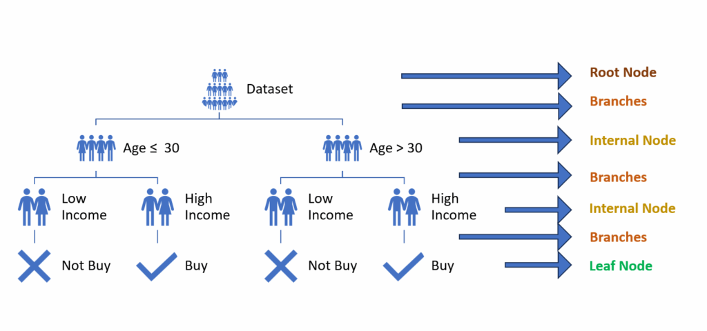
The elements that make up the Decision Tree are:

Root node: The main trunk of the tree from which all decisions originate. It contains the entire dataset used for the first split.

Internal nodes: These result from splitting the main dataset. The split typically occurs based on a condition (for example, dividing the dataset based on whether feature X is present or absent). These nodes separate the dataset into more refined, “pure” parts.

Branches: These connections between nodes represent the outcome of a split. They can lead either to new internal nodes or to leaves.

Leaf nodes: These final nodes represent the decision tree’s output, whether for classification (returning a label) or regression (returning a number). No further splits occur after leaf nodes.

Consider this example of a decision tree: Imagine a dataset with features like “Age” and “Income” that predicts whether someone will purchase a product (“buy” or “don’t buy”). The root node contains the complete dataset. The first split divides the data by age (< 30 years and ≥ 30 years), creating two branches leading to internal nodes. Each of these nodes then splits based on income level (“high income” and “low income”), leading to leaf nodes that provide the final decision (“buy” or “don’t buy”).

Building a Decision Tree: purity

How does the dataset separation occur at the nodes? The key element is purity—the dataset is divided at nodes to achieve maximum possible purity. Purity means how homogeneous the instances are within a dataset segment relative to the target. A pure node contains instances of only one class (for example, all “buy” decisions). An impure node, on the other hand, contains instances of different classes (both “buy” and “don’t buy” decisions).

Purity can be measured using several metrics:

Gini Impurity

The Gini index measures how likely an instance is to be misclassified at a node.

The formula is:

$Gini = 1 - \sum_{i=1}^{c} p_i^2$

where $p_i$ represents the probability of class i.

The Gini index equals 0 for a pure node (perfect classification), while for a highly impure node with an even 50-50 split between two classes, it equals 0.5.

Entropy

Entropy measures the randomness or disorder in a system—a higher entropy value indicates a more impure node.

The formula for calculating entropy is:

$Entropy = - \sum_{i=1}^{c} p_i \log_2(p_i)$

Here, $p_i$ represents the probability of class i in the node.

An entropy value of 0 indicates a pure node, while a value of 1 indicates an even split (50% of instances per class in a two-class classification).

Error Rate

The error rate measures the proportion of instances that are incorrectly classified at a node.

The formula is:

$Error\ Rate = 1 - \max(p_i)$

This metric is less commonly used than Gini impurity or entropy because it provides less detailed information about node purity.

Information gain

Our objective is to segment the dataset so that the purity of nodes concerning the target variable is maximized.

To optimize node purity, we evaluate potential splits in the dataset at each node level by calculating the information gain.

Information gain helps us determine if splitting the dataset on a particular feature will improve our metrics.

By evaluating each potential feature, we can identify which split will yield the best improvement in our decision tree.

Information Gain is calculated as:

$IG = I(parent) - \sum_{j} \frac{|D_j|}{|D|} I(D_j)$

Where:

• I(parent) represents the entropy of the node before splitting

• Dj represents the entropy of the resulting subsets

• Dj/D represents the proportion of data in each subset

When information gain equals zero, splitting on that feature provides no benefit. However, a high information gain indicates that the split will significantly improve node purity.

Numerical Example

Consider a small dataset of 6 patients where the target variable (risk assessment) shows 3 low-risk and 3 high-risk patients.

Let’s calculate the entropy of the root node.

$Entropy(parent) = - \left(\frac{3}{6} \log_2 \frac{3}{6} + \frac{3}{6} \log_2 \frac{3}{6} \right)$

$= - (0.5 \times \log_2 0.5 + 0.5 \times \log_2 0.5) = 1.0$

We can also calculate the Gini impurity of the root node:

$Gini(parent) = 1 - \left(\left(\frac{3}{6}\right)^2 + \left(\frac{3}{6}\right)^2\right)$

$= 1 - (0.25 + 0.25) = 0.5$

Let’s split the root node using cholesterol as our feature. The right node will contain patients with low cholesterol (≤ 200 mg/dl), and the left node will contain patients with high cholesterol (> 200 mg/dl).

All three patients in the right node have low cholesterol and are low risk, while all three patients in the left node have high cholesterol and are high risk.

These internal nodes are pure, meaning they contain only one class each.

Now let’s calculate the information gain from this split using both entropy and Gini impurity metrics.

First, the entropy of the child nodes:

$Entropy(left) = - \left(\frac{3}{3} \log_2 \frac{3}{3} + 0 \right) = 0$

$Entropy(right) = - \left(\frac{3}{3} \log_2 \frac{3}{3} + 0 \right) = 0$

Gini impurity in the child nodes:

$Gini(left) = 1 - \left(\frac{3}{3}\right)^2 = 0$

$Gini(right) = 1 - \left(\frac{3}{3}\right)^2 = 0$

The child nodes demonstrate perfect purity in terms of both entropy and Gini impurity metrics, with both values reaching zero. This occurs because each child node exhibits complete homogeneity in its composition—containing exclusively instances belonging to a single target class. When a node achieves this level of purity, it means there is no mixture or uncertainty in the classification of its instances, making it an ideal outcome in decision tree splitting. This perfect separation indicates that the chosen split criterion has effectively partitioned the data into clearly distinguished groups.

The entropy-based information gain:

$IG = Entropy(parent) - \left(\frac{3}{6} \times Entropy(left) + \frac{3}{6} \times Entropy(right) \right)$

$= 1.0 - (0.5 \times 0 + 0.5 \times 0) = 1.0$

An information gain of 1 indicates we’ve achieved the maximum possible improvement.

The Gini impurity-based information gain:

$IG = Gini(parent) - \left(\frac{3}{6} \times Gini(left) + \frac{3}{6} \times Gini(right) \right)$

$= 0.5 - (0.5 \times 0 + 0.5 \times 0) = 0.5$

This positive information gain confirms that our split effectively separates the classes.

Thus, cholesterol proves to be an effective feature for splitting the root node.

When we calculate information gain for other available features, we find:

Feature	Information Gain
Cholesterol	0.97
Blood Pressure	0.97
Age	0.42

Given these results, either cholesterol or blood pressure would be equally good choices for splitting, as they both have high information gain. Age, with its lower information gain, would be a less effective choice.

Choosing the Cutoff for Feature Division

In the example above, we used 200 mg/dl as the cutoff to divide patients based on cholesterol values. How do we determine the optimal threshold value to split a continuous variable into two groups?

This evaluation is crucial in decision trees. The process involves testing all possible values of a feature as potential cutoffs. We calculate the impurity for each potential threshold and select the one that yields the maximum information gain.

# Function to find the best cutoff for a feature using Entropy
def best_cutoff_entropy(X, y, feature):
    sorted_values = np.sort(X[feature].unique())  # Sort the feature values
    best_cutoff, best_IG = None, -np.inf
    
    for i in range(len(sorted_values) - 1):
        cutoff = (sorted_values[i] + sorted_values[i + 1]) / 2  # Average between two consecutive values
        left_y = y[X[feature] <= cutoff]  # Left subset
        right_y = y[X[feature] > cutoff]  # Right subset

        # Calculate entropy of both subsets
        entropy_left = entropy(left_y)
        entropy_right = entropy(right_y)
        
        # Weight the entropy based on group sizes
        n_left, n_right = len(left_y), len(right_y)
        weighted_entropy = (n_left / len(y)) * entropy_left + (n_right / len(y)) * entropy_right
        
        # Information Gain
        IG = entropy(y) - weighted_entropy
        
        # Update the best cutoff
        if IG > best_IG:
            best_IG = IG
            best_cutoff = cutoff
    
    return best_cutoff, best_IG

# Find the best cutoff for the "Cholesterol" feature
best_cutoff_chol, best_IG_chol = best_cutoff_entropy(X_complex, y_complex, "Cholesterol")
best_cutoff_chol, best_IG_chol

# Function to find the best cutoff for a feature using Entropy
def best_cutoff_entropy(X, y, feature):
    sorted_values = np.sort(X[feature].unique())  # Sort the feature values
    best_cutoff, best_IG = None, -np.inf
    
    for i in range(len(sorted_values) - 1):
        cutoff = (sorted_values[i] + sorted_values[i + 1]) / 2  # Average between two consecutive values
        left_y = y[X[feature] <= cutoff]  # Left subset
        right_y = y[X[feature] > cutoff]  # Right subset

        # Calculate entropy of both subsets
        entropy_left = entropy(left_y)
        entropy_right = entropy(right_y)
        
        # Weight the entropy based on group sizes
        n_left, n_right = len(left_y), len(right_y)
        weighted_entropy = (n_left / len(y)) * entropy_left + (n_right / len(y)) * entropy_right
        
        # Information Gain
        IG = entropy(y) - weighted_entropy
        
        # Update the best cutoff
        if IG > best_IG:
            best_IG = IG
            best_cutoff = cutoff
    
    return best_cutoff, best_IG

# Find the best cutoff for the "Cholesterol" feature
best_cutoff_chol, best_IG_chol = best_cutoff_entropy(X_complex, y_complex, "Cholesterol")
best_cutoff_chol, best_IG_chol

This will give us the indication of the best cholesterol value to use as a cutoff (for example 215 mg/dl) which corresponds to the best information gain value (example 0.8).

Medical Applications of Decision Trees

Decision trees have emerged as powerful analytical tools with numerous valuable applications across various medical domains and healthcare settings:

Disease diagnosis: Using structured branching logic to systematically analyze and group clinical indicators, symptoms, and test results to assist healthcare providers in reaching accurate diagnoses efficiently

Risk stratification: Identifying high-risk patients through comprehensive analysis of key characteristics, including demographic factors, medical history, lifestyle choices, and current health metrics to enable proactive interventions.

Mortality prediction: Assessing likelihood of patient outcomes by evaluating complex combinations of vital signs, laboratory values, comorbidities, and treatment responses to guide clinical decision-making

Clinical decision support: Guiding healthcare providers through evidence-based choices by integrating current medical knowledge, established clinical guidelines, and patient-specific data to optimize treatment plans and improve care delivery

There are many works in the medical literature that use implementations of these models:

Batterham PJ, Christensen H, Mackinnon AJ. Modifiable risk factors predicting major depressive disorder at four-year follow-up: a decision tree approach. BMC Psychiatry. 2009;9:75. doi: 10.1186/1471-244X-9-75)

Li C, Gluer CC, Eastell R, Felsenberg D, Reid DM, Rox DM, Lu Y. Tree-structured subgroup analysis of receiver operating characteristic curves for diagnostic tests. Acad Radiol. 2012;19(12): 1529–1536. doi: 10.1016/j.acra.2012.09.007

Maheswari S, Pitchai R. Heart Disease Prediction System Using Decision Tree and Naive Bayes Algorithm. Curr Med Imaging Rev. 2019;15(8):712-717. doi: 10.2174/1573405614666180322141259. PMID: 32008540.

Bamber JH, Evans SA. The value of decision tree analysis in planning anaesthetic care in obstetrics. Int J Obstet Anesth. 2016 Aug;27:55-61. doi: 10.1016/j.ijoa.2016.02.007. Epub 2016 Feb 27. PMID: 27026589.

Wang L, Zhu L, Jiang J, Wang L, Ni W. Decision tree analysis for evaluating disease activity in patients with rheumatoid arthritis. J Int Med Res. 2021 Oct;49(10):3000605211053232. doi: 10.1177/03000605211053232. PMID: 34670422; PMCID: PMC8543724.

Huang H, Yang ZH, Gu ZW, Luo M, Xu L. Decision Tree Model for Predicting the Overall Survival of Patients with Diffused Large B-Cell Lymphoma in the Central Nervous System. World Neurosurg. 2022 Oct;166:e189-e198. doi: 10.1016/j.wneu.2022.06.139. Epub 2022 Jul 5. PMID: 35803570.

When to Use Decision Tree

The decision tree algorithm demonstrates particular effectiveness in scenarios where data exhibits clear patterns that can be segmented through decision rules. It excels when working with datasets that naturally follow a hierarchical or tree-like structure, where decisions flow logically from one level to the next. This algorithm is especially well-suited for smaller datasets where the relationships between variables are relatively simple and interpretable, making it an ideal choice when transparency in decision-making processes is crucial and when the data volume remains manageable without requiring complex computational resources.

Limitations of using Decision Tree

Decision trees should be used with caution when dealing with highly variable datasets or those containing numerous features, as these conditions significantly increase the risk of overfitting. In such scenarios, the tree may become too complex and specific to the training data, leading to poor generalization when applied to new, unseen cases. This limitation becomes particularly pronounced when the dataset exhibits high dimensionality or contains substantial noise in the feature space.

Another important consideration is that decision trees may not be the optimal choice for applications requiring continuous predictions or scenarios demanding extremely high accuracy levels. The discrete nature of tree-based predictions, which segment data into distinct branches and leaves, can result in less precise outputs compared to other machine learning models designed specifically for continuous variable prediction. This stepwise prediction pattern may not capture subtle variations in the target variable, making them less suitable for problems where precise, granular predictions are essential.

Implementing Decision Trees in Python

To build Decision Trees in Python, you’ll use the scikit-learn tree library. It offers two main classes: DecisionTreeClassifier for classification problems and DecisionTreeRegressor for regression problems.

These models require specific hyperparameters that shape the tree’s structure and influence its performance.

The key hyperparameters include:

criterion: determines how node purity is evaluated
- for classification: “gini” or “entropy”
- for regression: “squared_error”, “friedman_mse”, “absolute_error”
max_depth: sets the tree’s maximum depth
- higher values may lead to overfitting
- lower values may cause underfitting
min_samples_split: sets the minimum samples needed to split a node
- defaults to 2
min_samples_leaf: sets the minimum samples required in a leaf node
- defaults to 1
max_leaf_nodes: maximum number of leaves allowed
class_weight: adjusts class weights for imbalanced datasets
- “balanced” option handles weighting automatically
splitter: chooses the data splitting method
- “best” optimizes information gain
- “random” splits data randomly

Let’s explore the “pruning” technique, which reduces decision tree complexity and prevents overfitting.

Pruning removes the least informative branches of a tree.

Pre-pruning occurs before training by setting hyperparameters that constrain tree growth (max_depth, min_samples_split, min_samples_leaf, max_leaf_nodes). However, this early intervention may prevent the model from discovering its optimal structure.

Post-pruning occurs after tree construction using Cost Complexity Pruning Alpha (ccp_alpha). This parameter adds a penalty term for each tree node—as ccp_alpha increases, more nodes are removed. While post-pruning allows full tree training before optimization, its main drawback is that the optimal ccp_alpha value must be determined through empirical testing.

For our medical risk assessment, we implemented the DecisionTreeClassifier on a simulated dataset.

The model evaluates three risk levels: “low”, “medium”, and “high”.

We visualize the results through both a decision tree diagram and a confusion matrix.

import numpy as np
import pandas as pd
import matplotlib.pyplot as plt
from sklearn.tree import DecisionTreeClassifier, plot_tree
from sklearn.model_selection import train_test_split
from sklearn.metrics import accuracy_score, classification_report, confusion_matrix
import seaborn as sns

# Generate a more complex medical dataset
np.random.seed(42)
n_samples = 500

data = pd.DataFrame({
    "Age": np.random.randint(30, 80, size=n_samples),
    "Cholesterol": np.random.randint(150, 300, size=n_samples),
    "Blood_Pressure": np.random.randint(90, 180, size=n_samples),
    "Diabetes": np.random.choice([0, 1], size=n_samples),  # 0: No, 1: Yes
    "Smoking": np.random.choice(["Never", "Former", "Current"], size=n_samples),
    "Obesity": np.random.choice(["Normal", "Overweight", "Obese"], size=n_samples),
    "Family_History": np.random.choice(["No", "Yes"], size=n_samples),
    "Risk": np.random.choice(["Low", "Medium", "High"], size=n_samples)  # Target variable
})

# Encoding categorical variables
from sklearn.preprocessing import LabelEncoder

label_encoders = {}
for col in ["Smoking", "Obesity", "Family_History", "Risk"]:
    le = LabelEncoder()
    data[col] = le.fit_transform(data[col])
    label_encoders[col] = le

# Splitting dataset
X = data.drop(columns=["Risk"])
y = data["Risk"]
X_train, X_test, y_train, y_test = train_test_split(X, y, test_size=0.2, random_state=42)

# Creating and training the Decision Tree model
clf = DecisionTreeClassifier(criterion="entropy", max_depth=5, random_state=42)
clf.fit(X_train, y_train)

# Predict and evaluate the model
y_pred = clf.predict(X_test)
accuracy = accuracy_score(y_test, y_pred)
print(f"Model Accuracy: {accuracy:.2f}")
print("Classification Report:\n", classification_report(y_test, y_pred))

# Plot the Decision Tree
plt.figure(figsize=(16, 10))
plot_tree(clf, feature_names=X.columns, class_names=["Low", "Medium", "High"], filled=True, fontsize=8)
plt.title("Complex Medical Decision Tree for Cardiovascular Risk")
plt.show()

# Confusion Matrix
conf_matrix = confusion_matrix(y_test, y_pred)
sns.heatmap(conf_matrix, annot=True, fmt="d", cmap="Blues", xticklabels=["Low", "Medium", "High"], yticklabels=["Low", "Medium", "High"])
plt.xlabel("Predicted")
plt.ylabel("Actual")
plt.title("Confusion Matrix")
plt.show()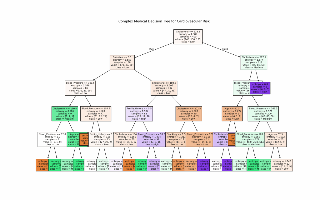

import numpy as np
import pandas as pd
import matplotlib.pyplot as plt
from sklearn.tree import DecisionTreeClassifier, plot_tree
from sklearn.model_selection import train_test_split
from sklearn.metrics import accuracy_score, classification_report, confusion_matrix
import seaborn as sns

# Generate a more complex medical dataset
np.random.seed(42)
n_samples = 500

data = pd.DataFrame({
    "Age": np.random.randint(30, 80, size=n_samples),
    "Cholesterol": np.random.randint(150, 300, size=n_samples),
    "Blood_Pressure": np.random.randint(90, 180, size=n_samples),
    "Diabetes": np.random.choice([0, 1], size=n_samples),  # 0: No, 1: Yes
    "Smoking": np.random.choice(["Never", "Former", "Current"], size=n_samples),
    "Obesity": np.random.choice(["Normal", "Overweight", "Obese"], size=n_samples),
    "Family_History": np.random.choice(["No", "Yes"], size=n_samples),
    "Risk": np.random.choice(["Low", "Medium", "High"], size=n_samples)  # Target variable
})

# Encoding categorical variables
from sklearn.preprocessing import LabelEncoder

label_encoders = {}
for col in ["Smoking", "Obesity", "Family_History", "Risk"]:
    le = LabelEncoder()
    data[col] = le.fit_transform(data[col])
    label_encoders[col] = le

# Splitting dataset
X = data.drop(columns=["Risk"])
y = data["Risk"]
X_train, X_test, y_train, y_test = train_test_split(X, y, test_size=0.2, random_state=42)

# Creating and training the Decision Tree model
clf = DecisionTreeClassifier(criterion="entropy", max_depth=5, random_state=42)
clf.fit(X_train, y_train)

# Predict and evaluate the model
y_pred = clf.predict(X_test)
accuracy = accuracy_score(y_test, y_pred)
print(f"Model Accuracy: {accuracy:.2f}")
print("Classification Report:\n", classification_report(y_test, y_pred))

# Plot the Decision Tree
plt.figure(figsize=(16, 10))
plot_tree(clf, feature_names=X.columns, class_names=["Low", "Medium", "High"], filled=True, fontsize=8)
plt.title("Complex Medical Decision Tree for Cardiovascular Risk")
plt.show()

# Confusion Matrix
conf_matrix = confusion_matrix(y_test, y_pred)
sns.heatmap(conf_matrix, annot=True, fmt="d", cmap="Blues", xticklabels=["Low", "Medium", "High"], yticklabels=["Low", "Medium", "High"])
plt.xlabel("Predicted")
plt.ylabel("Actual")
plt.title("Confusion Matrix")
plt.show()

Complex medical decision tree for cardiovascular risk

Conclusion

The Decision Tree is one of the most intuitive and interpretable Machine Learning algorithms, providing a clear hierarchical structure for data-driven decisions. Though it has limitations with complex datasets and tends to overfit, it excels as a powerful tool for classification and regression tasks—particularly in fields like medicine where model transparency is crucial.